Analysis Functions
Cook disordered
Before hands-on with the Pathway or SWR pipelines, please be patient
with this gentle introduction about the cook_disordered function.
The SWR, binding energy and part of the Pathway analysis are built on
top of this function. Since it’s convenient to use, the results are
highly informative and structural.
It was July 2022, we were working on the pathway analysis. Initially, we performed the routine refinement procedure of pathways. That is, start from the 10-kilo NNP pathways to the 1-kilo xTB pathways and finally come to the 100 DFT pathways. Back then, we are excited about what we have found. However, after carefully reviewing our results, we found that this refinement procedure is still not perfect. See Fig 1. From a topological view, the C60Cl4-2 adduct is the same as C60Cl4-1. However, when it comes to pathway search, only C60Cl4-1 will take accounted as one of the C60Cl6 precursors, meanwhile, C60Cl4-2 will be thrown away. Although this scenario will not happen because we have adopted usenauty to enumerate non-isomorphic patterns. The point is that some topological information has been lost during the simulation procedure, resulting in connections like C60Cl6 and C60Cl4-2 will never be considered in the later analysis workflows.
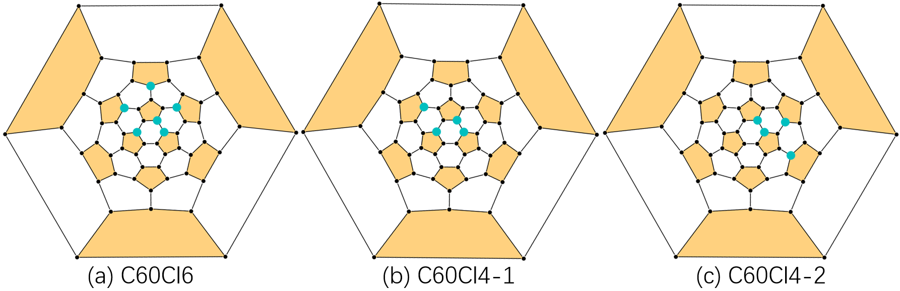
Fig 1. The problem of pathway search.
To properly address this problem, we developed the get_connection
function to re-generate topological information for a small batch of
isomers (by NetworkX
Isomorphism
module). Since this function requires highly structured inputs, we
developed the simple_parse_logs function to properly parse and
sort legacy simulation data. Following these two functions, a
pathway search program is immediately developed. Fig 2 sums up the
cook_disordered pipeline and its capabilities. Since most of the
computation cost comes from the get_connection function for solving
sub-graph isomorphism problems, we do not recommend applying this
function for huge batches of isomers. 100 or some DFT results will be
acceptable.
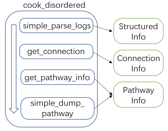
Fig 2. The cook_disordered pipeline and its capabilities.
To use it, one needs to provide the following parameters:
disordered_root: path to the disordered root. It could be any of your legacy DFT (xTB) results, simply copying and pasting them to one folder and naming this folderdisordered_rootwill be good. Note that, equal addon intervals are required. It could be 1_addons, 2_addons or 2_addons, 4_addons. The program will be broken for 1, 2, 4 scenarios.step: the step, the addon interval.file_mid_name: to customize the filename (optional). Currently, the filename convention consists of two info. For example, 2_addons_2, 1 means the number of addends, 2 means this isomer ranks 2 in all considered C2nX2. This parameter will insert new flags into the name convention. For example, iffile_mid_name=xtb_rank, the results could be2_addons_xtb_rank_2. The phaseaddonsis a fixed mid filename.dump_root: path to dump information.keep_top_k_pathway: how many generated pathways to keep. (in rank mode)log_mode: two log formats are supported. 1. the Gaussian format, type the keywordgauss. 2. the xyz format, type the keywordxtb.has_pathway: set false to skip pathway generation. By default, this is true, since pathway search on a small batch of isomers is extremely easy.
For an example, see
cook_disordered.
Fig 3 presents the cook_disordered results. The sorted folder
contains the structured information we need for SWR analysis or binding
energy analysis.
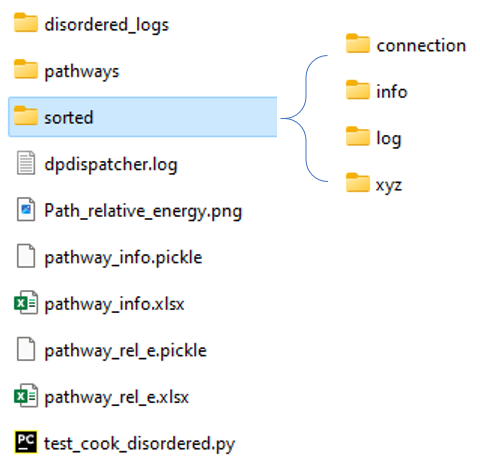
Fig 3. The cook disordered workbase.
It contains the following results:
./sorted/log: the final (typically) optimization logs for a specific isomer. File names contain two metrics. The first number means the number of addends, the last number means the ranking of the specific isomer. For example,1_addons_1means it contains 1 addend and its energy rank is 1 (the lowest energy one)../sorted/xyz: the final image of the optimization trajectory. The name convention is the same as above../sorted/info: energy information. (in pickle and excel format)./sorted/connection: connection information.1_addons_1.npycorresponds to the isomer, whose geometry information is stored in1_addons_1.xyz. This isomer has connection relationships with higher addends, here, in this case, it means 2 addends.1_addons_1.npystores this information, 1 meaning connected, 0 for not.
Note that, if one is pursuing numerical addon labels like 1_2_31,
please check Plot_With_FullereneDataParser. It will give a better
visualization.
Path parser
The development of the path parser abstraction started from the very
beginning of AutoSteper. It was noted that when a pattern “gives birth
to” a new pattern, there exists a topological bond between the
two. For example, an isomer with an addon pattern [0, 1] may have a
derivative with an addon pattern [0, 1, 3]. This corresponds to the
step mode of usenauty module. During the build-on-the-fly procedure,
this kind of topological information will be stored as a by-product of
the growth simulation. Here we name this kind of information as
parent-son information and store it in the parent_info.pickle.
The early version of the pathway search program is built to parse this
information. With no need to generate topological connection
information, this program is extremely fast. However, as mentioned in
the previous section, the parent-son information is incomplete from the
topological view, whereafter we built another pathway search program
based on the re-generated connection information (by NetworkX
Isomorphism
module), yet this program can only be applicated to a small batch of
isomers since solving subgraph isomorphism problem is expensive.
The programs mentioned above have been wrapped into a single
abstraction, Path_Parser. Next, we present an introduction to each
of its methods.
get_path_from_sim
This method will parse simulation-generated parent_son information. One may follow the script below:
import os

from autosteper.parser import Path_Parser


a_path_parser = Path_Parser()
a_path_parser.get_path_from_sim(dump_root=r'path/to/sim_pathways',
                                pristine_cage_path=r'path/to/C60.xyz',
                                sim_workbase=r'path/to/C60',
                                sim_step=1, sim_start=1, q_add_num=6, q_path_rank=5, q_isomer_rank=3,
                                is_mix=True)
Here is a short explanation of each parameter:
dump_root: which folder to dumppristine_cage_path: path to pristine cagesim_xx: simulation-related parameters, same as the run parameters.q_xx: query atoms related parameters. To start with, the formula \(\rm C_{2n}X_{m}\_i\) is for the isomer of cage size 2n, addon number m, and energy rank i. For pathway search of it, one may type keywordsq_add_num=m, andq_isomer_rank=i. The cage size 2n has been calculated from the pristine cage.q_path_rankmeans how many pathways to dump, in the format of heatmap and xyz files.is_mix: this parameter is for the query of multiple end-addition-state isomers. By default, this parameter will be false. The query will be focused on a specific end-addition-state isomer. Set this parameter to true will enable query for all \(\rm C_{2n}X_{m}\_i, i<=q\_isomer\_rank\) isomers.is_ctr_path: set this parameter to true to control the scale of pathways. As mentioned above, the pattern [0, 1, 3] may have a parent pattern [0, 1]. In fact, there may exist another parent pattern [0, 3], which is NOT isomorphic with [0, 1]. Both of them will give birth to [0, 1, 3]. Therefore, pattern [0, 1, 3] will have two parents. This is the key to controlling the number of generated pathways. Sinceget_path_from_simis a DFS program, limiting the number of parents will bring the pathway search manageable. The parameterctl_parent_numwill clean the parent_info.pickle file by sorting parents with energy rank and throwing away high-energy parents. Additionally, the parametermax_path_numwill set an upper limit to theraw_pathway_info.picklefile. These parameters are helpful for query isomers with high addends, say 20 or 30. The results may reach half a million. It’s recommended to setctl_parent_numas 2 or 1 and setmax_path_numto 10000.
The results of this method are presented below:
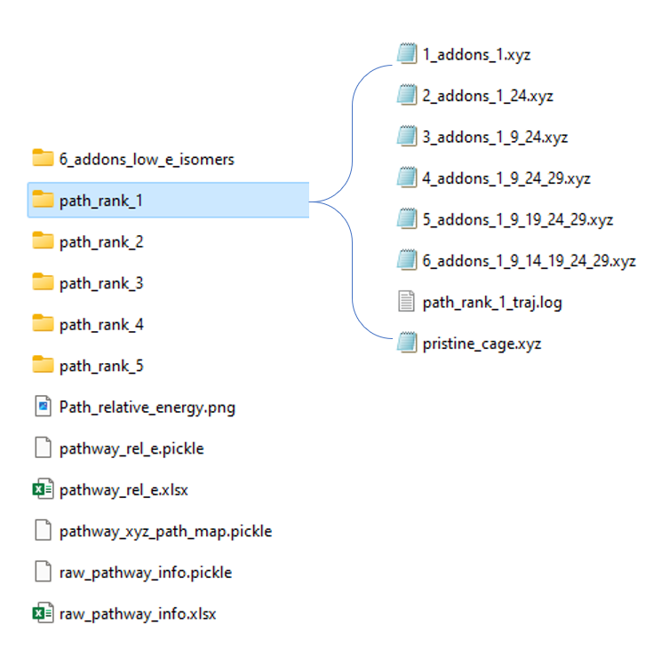
Fig 4. Folder system for get_path_from_sim results.
The folder system has been refactored recently for a general readership. For each pathway result P_i, i <= q_path_rank, there will be a unique folder named path_rank_i created. This folder lists pathway-related isomers in xyz format. And a log file for dynamic visualization. (ASE GUI)
The energy differences between pathways and isomers are summed up into the heatmap:
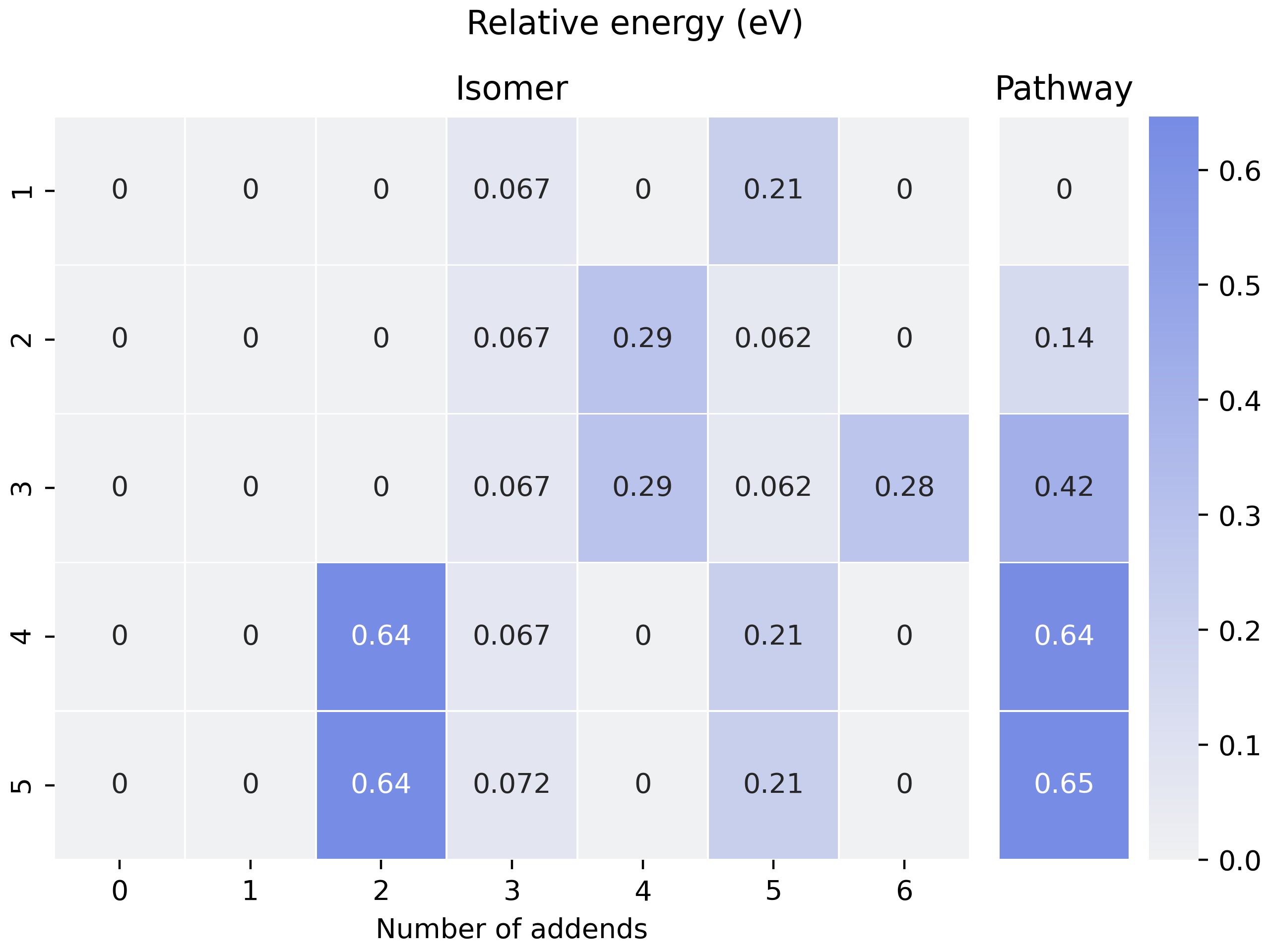
Fig 5. Heatmap for visualization of pathways.
In this heatmap, each row is a unique pathway, and columns on the
sub-figure Isomer mean the number of addends. The split column is for
the relative energy of pathways. It is indeed the sum up of the left
sub-figure, though it has deviated from our original planning. As one
may notice in the raw_pathway_info.xlsx, the name of this column is
e_area. This is the deprecated name of ‘Pathway’ in Fig 5. In fact,
we are planning to compare different pathways by the surrounding area
like activation energy curves in catalyst research initially, see Fig 6.
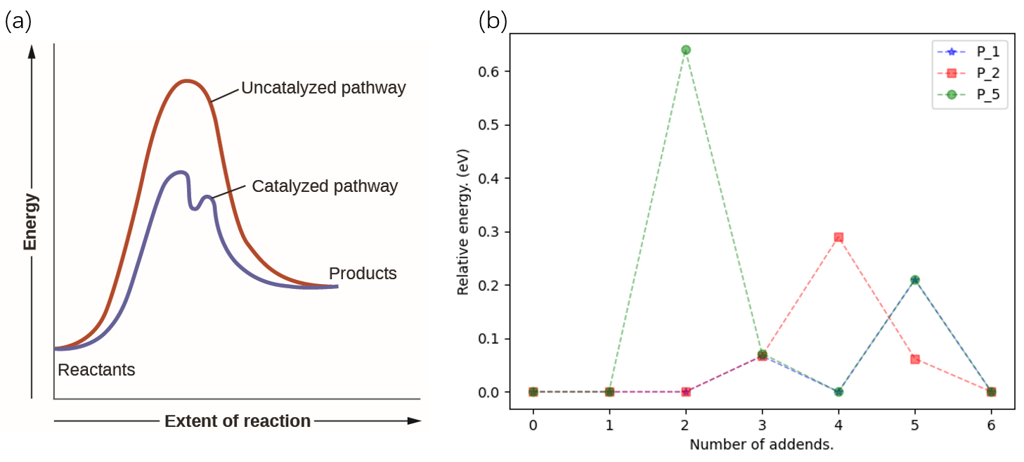
Fig 6. Illustration of the e-area concept.
It’s much more convincing for the general readership if we compare pathways by area. An area solver is quickly developed, say, we add two triangles surrounded by the first and last relative E, as well as the trapezoids surrounded by intermediates. We will have equation (1) as below. Here we set the base of a triangle and the height of a trapezoid to a constant \(C\).
Here equation (1) is simplified to equation (2). So, after a whole roundabout, we come back to the criterion of a simple sum up.
update_path_info
Humanity’s pursuit of computational accuracy is never-ending. Here for the pathway search scenario, the update of evaluators may be desired. For example, from NNP to xTB, and then, from xTB to DFT.
To do this, one may follow the script below, input parameters are easy to understand:
import os

from autosteper.parser import Path_Parser

refiner_para = {autosteper.optimizer parameters}

a_path_parser = Path_Parser()
a_path_parser.update_path_info(old_workbase=r'path/to/sim_pathways',
                               new_workbase=r'path/to/updated_sim_pathways',
                               refine_top_k=4,
                               refine_mode='xtb',
                               refiner_para=refiner_para)
This will update pathway info with a higher level of computation method.
re_generate_pathways
After the multi-level refinement procedure, there would be much fewer
pathways on hand. As mentioned in the cook_disordered section, we
are capable to do a complete pathway search with all the topological
connections considered. Therefore, this method is a simple wrapper of
cook_disordered function. To use it, one may follow the script as
below:
import os

from autosteper.parser import Path_Parser


a_path_parser = Path_Parser()
a_path_parser.re_generate_pathways(old_workbase=r'path/to/updated_sim_pathways',
                                   new_workbase=r'path/to/regenerated_pathways',
                                   step=1, last_log_mode='xtb', keep_top_k_pathway=3, group='Cl')
Note that, the re-generated pathway may look disordered in terms of
numerical labels. For example, a pattern [0, 1] can have a son [1, 2,
3]. For a general readership, the filename convention of re-generated
pathways follows the 1_addons_1 as mentioned above. For a better
visualization, please check the PlotWithFullerneDataParser section.
The recommended workflow
Here in Fig 7, we present the recommended workflow for pathway search.
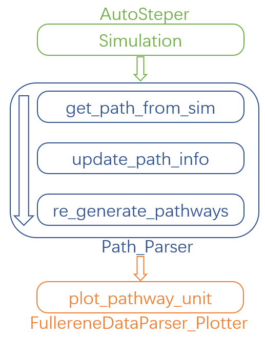
Fig 7. The recommended pathway search workflow.
That is:
Perform a growth simulation with AutoSteper to get enough intermediates for the queried atoms.
Get pathways from topological information generated along with the simulation.
Update evaluators to a higher computational method. This procedure may be performed repeatedly.
Re-generate complete topological information and perform a complete pathway search within remaining isomers.
Visualize pathways with FullereneDataParser_Plotter.
SWR analysis
The Stone-Wales rearrangement (SWR) in fullerene chemistry is like gene mutation in biology. A SWR takes place on a cage means there is at least one C-C bond that takes a 90° rotation, and changes this cage to a more chemically active or stable one. As gene mutation does for DNA.
It has been a widely observed phenomenon that functional groups could significantly activate the to-be-rotated C-C bond. Based on this observation, we developed an SWR search program. Specifically, we focus on the mid-addition stage. Two topological rules and one energy criterion have been established to screen the possible SWR scenarios. For description convenience, here we denote an isomer before and after the SWR as \(\rm ^{\#1}C_{2n}Cl_{2m}\) and \(\rm ^{\#2}C_{2n}Cl_{2(m+1)}\).
That is:
At least one of the four sites around the rotated C-C bond should be occupied during the SWR process.
The \(\rm ^{\#1}C_{2n}Cl_{2m}\) structure should be a subgraph of \(\rm ^{\#2}C_{2n}Cl_{2(m+1)}\) when excluding the rotated C-C bond.
The \(\rm ^{\#1}C_{2n}Cl_{2m}\) may have multiple SWR products \(\rm ^{\#2}C_{2n}Cl_{2(m+1)}\), the lowest energy one should have lower energy than the competitive \(\rm ^{\#1}C_{2n}Cl_{2(m+1)}\) products. (Optional)
Note that, in the practical SWR search, there are much more tricky exceptions to be dealt with. Almost all of them came from unexpected isomorphism problems. Fig 8 presents two of the screened SWR results:
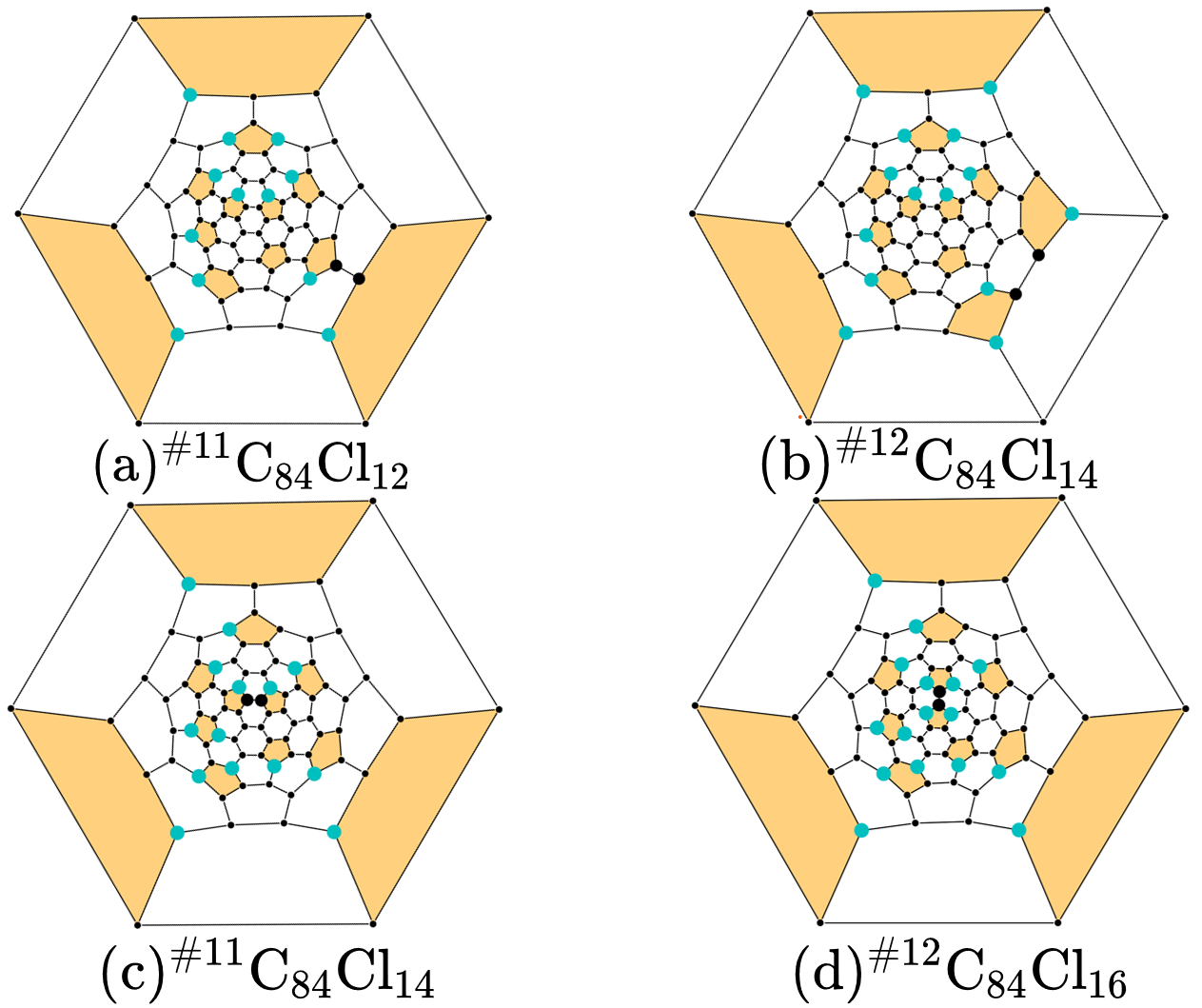
Fig 8. Visualization of the isomorphism problem.
There is indeed one SWR step between cage \(\rm ^{\#11}C_{84}\) and \(\rm ^{\#12}C_{84}\). However, from a topological view, there are two SWR pairs found to exist. Or in other words, these two pairs point to the same C-C bond rotation, but in different labels.
After careful refactoring and extensive testing, in the latest version of AutoSteper, this problem has been fixed. And an automated pipeline has been built to wrap the whole SWR analysis into a single function. Although we still recommend users read through the inner part of this pipeline to get a more general view.
find SWR
This is the main SWR search program, it was designed as follows:
map pristine cages to find SWR pairs (on the cage level).
map the target system to the query system with two topological rules and one energy criterion considered.
re-label the target system (shuffle carbon atoms) to have an identical carbon sequence except for the SWR sites. This is for the visualization convenience.
To applicate this program, the cook_disordered function is required
to have structural information prepared.After that, one may follow the
script below:
import os

from autosteper.parser import find_SWR


find_SWR(q_sorted_root=r'./cook_disordered_results/11_C84_cooked',
         tgt_sorted_root=r'./cook_disordered_results/12_C84_cooked',
         swr_dump_path=r'./q_11_to_tgt_12',
         is_unique=True,
         is_low_e=True)
Two of the parameters need to be taken carefully:
is_low_e: set true to enable an energy criterionis_unique: set true to keep only one SWR product
The SWR results are highly structured, see Fig 9:
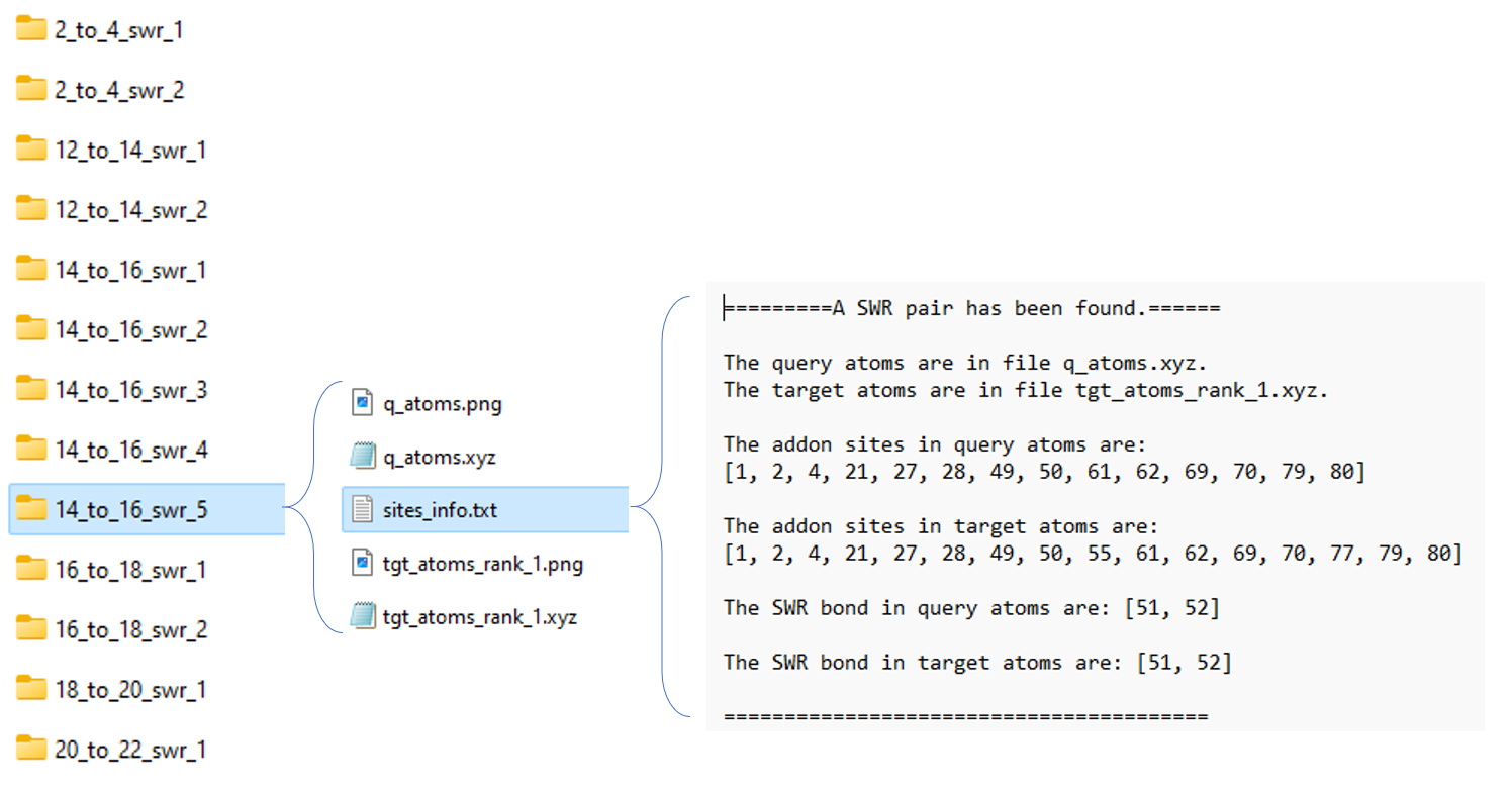
Fig 9. Folder system for SWR search results.
From left to right:
14_to_16_swr_5: this means the queried isomer has 14 addends while the target isomer has 16 addends. The final numerical label 5 means the queried isomers have an energy rank of 5 among other queried isomers.Note, for each queried isomer, there may be more than one target isomer that met the rules mentioned above. If the flag
is_uniqueis set to True, only one of the target isomers will be saved. (The lowest energy one) There are pictures to visualize this SWR pair, we will describe it later.site_info.txt: it stores detailed site information.
Count SWR
As one may notice, the SWR search results are kind of tricky to follow. So, what can we do with this messy data?
Well, let’s start with the sub-folders in Fig 10, one may notice that, there are more than one SWR pairs detected from \(\rm ^{\#11}C_{84}Cl_{14}\) and \(\rm ^{\#12}C_{84}Cl_{16}\) (5 in total). That is, 5 \(\rm ^{\#11}C_{84}Cl_{14}\) lowest energy isomers will have a tendency to transform to \(\rm ^{\#12}C_{84}Cl_{16}\). Simply counting these numbers will give a general view. Additionally, \(\rm ^{\#11}C_{84}\) could transform to \(\rm ^{\#12}C_{84}\), then, how about the reverse, \(\rm ^{\#12}C_{84}\) to \(\rm ^{\#11}C_{84}\)? If we search SWR pairs for both scenarios and compare them. This will reveal new insights into the interplay.
Considering that, we developed a simple counting program count_SWR
to compare SWR between two systems.
To use this function, one needs to provide the following parameters:
swr_1_legend: legend of theswr_1swr_2_legend: legend of theswr_2swr_1_workbase: output offind_SWRswr_2_workbase: samedump_pic_path: absolute path to the final picture.
For script, see SWR example.
Here is an example of an SWR count. It compares the SWRs between \(\rm ^{\#11}C_{84}Cl_x\) and \(\rm ^{\#12}C_{84}Cl_{x+2}\). For example, in the x=2 stage, there are 8 SWRs detected from \(\rm ^{\#11}C_{84}Cl_2\) to \(\rm ^{\#12}C_{84}Cl_4\), and when it comes to the post-addition stage, this number went to zero.
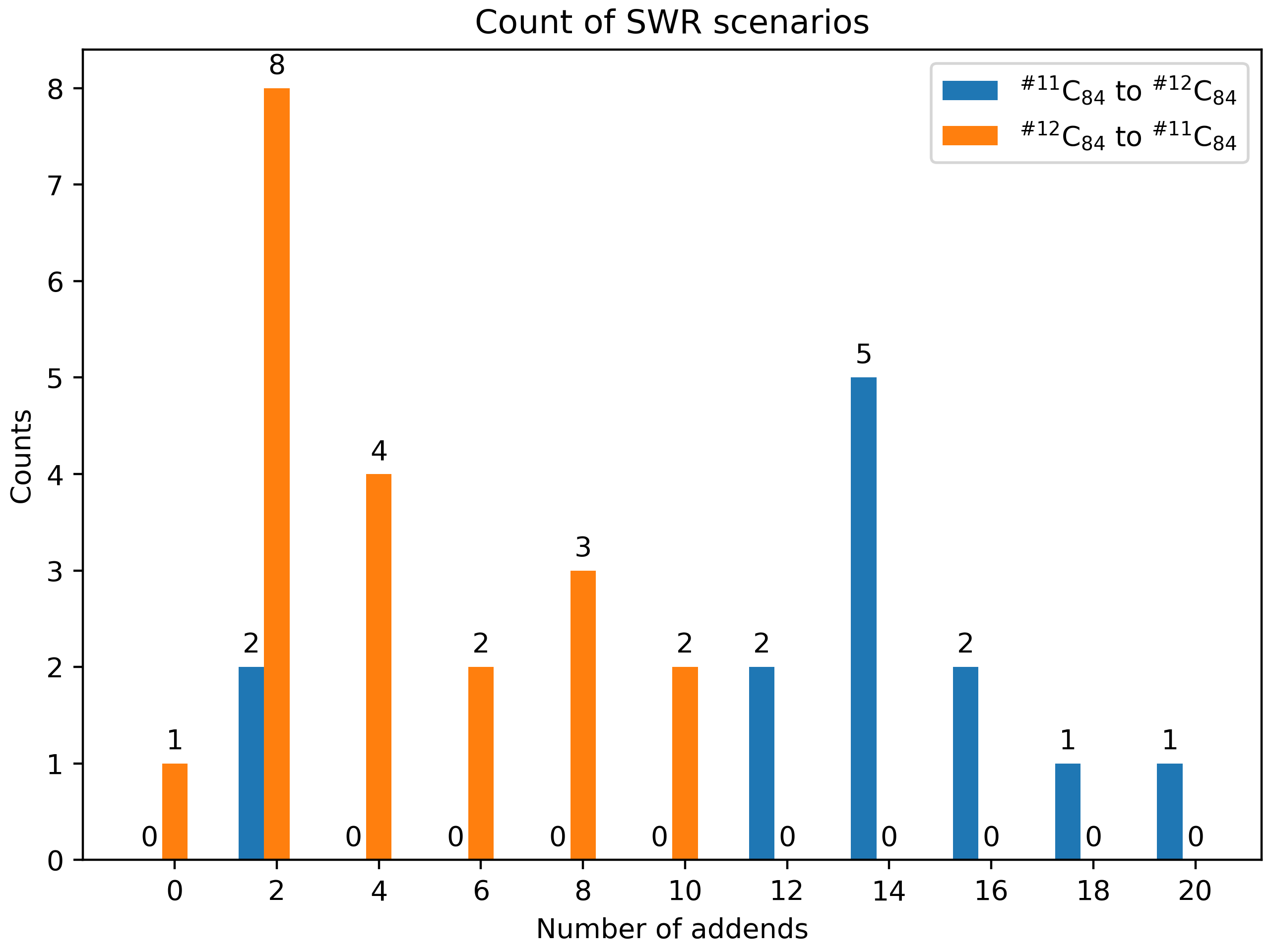
Fig 11. Illustration of SWR counts.
The recommended workflow
Here in Fig 12, we present the recommended workflow for SWR analysis.
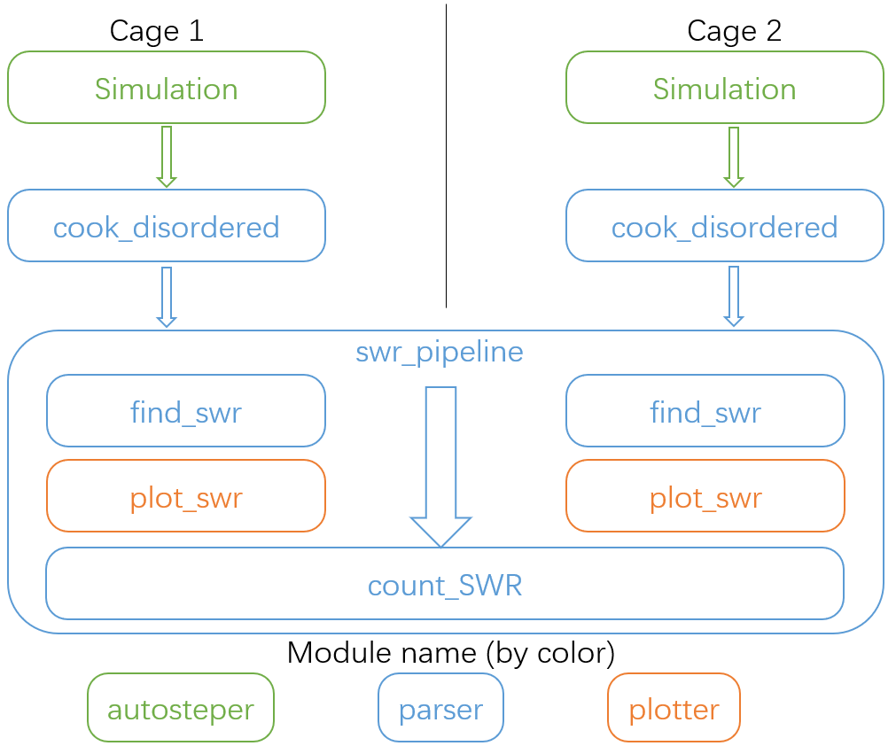
Fig 12. The recommended workflow for SWR analysis.
That is:
Perform growth simulation on two pristine cages with AutoSteper.
After refinement of simulation results, re-generate topological linkage information with
cook_disorderedfunction.Send structured results to the SWR pipeline to find, plot, and count SWR pairs.
Refine
When one needs to improve computational accuracy for growth simulation,
the refine function in the parser module presents a nice
solution. Only 3 parameters are needed to perform a refinement
procedure. That is:
old_workbase: the original workbase.new_workbase: the new workbase.ref_para: the same format as the optimizer’s parameter to configure an optimizer.
That’s it. AutoSteper will refine the original data and dump them into the new workbase. For details, see test_refine.py.
Isomorphism test
AutoSteper provides 3 functions to perform the isomorphism test. For example, see isomorphism.
Details are presented below:
simple_test_iso
This function is designed to test whether a specific isomer \(\rm ^{\#M}C_{2n}X_{m}\) is within the simulation results \(\rm ^{\#M}C_{2n}X_{m}\_q,0<q<=max\_rank\). If it’s indeed within the results, this function will output its corresponding rank \(\rm q\). One needs to provide:
q_atoms: the queried isomer, in ASE Atoms format.passed_info_path: the absolute path to the queriedpassed_info.pickle.top_k: a cutoff performed on thepassed_info.pickle,rankmode only. If none, AutoSteper will scan all the simulation results.
simple_log_relatives
This function is designed to quickly find relatives of a specific isomer \(\rm ^{\#M}C_{2n}X_{m}\) and log key information to a writeable path. Here relatives mean the intermediates (\(\rm ^{\#M}C_{2n}X_{q}, q<m\)), isomer (\(\rm ^{\#M}C_{2n}X_{q}, q=m\)) and derivatives (\(\rm ^{\#M}C_{2n}X_{q}, q>m\)) of the queried isomer. To ensure a fast test, here use the addition patterns as a criterion.
Two ways to decide the queried addition pattern.
The recommended way to get the addition pattern:
q_atoms: the queried isomer, in ASE Atoms format. Note that, it needs to have an identical pristine cage to the target. This ensures an identical sequence.group: the symbol of the functional group.cage_size: the size of the pristine cage.
The second way to get the addition pattern:
q_seq: the 36-base format name. See the 36 base function.q_cage: the key to decipher the 36-base name to a sequence, in AutoSteper/cage format.
After that, one needs to provide:
fst_add_num: the smallest addon number to be scanned.final_add_num: the biggest addon number to be scanned.step: the step that used in the growth simulation.workbase: the original workbase.dump_log_path: the absolute path to dump the related information.
Here is an example of the dumped log.
strict_scatter_relatives
This function is designed to strictly find relatives of a specific isomer. It implements the subgraph_is_isomorphic function to perform the isomorphism test and dump information in a png format (see Fig 13). The input parameters are basically the same as the above function. The difference is that it needs a folder to dump information.
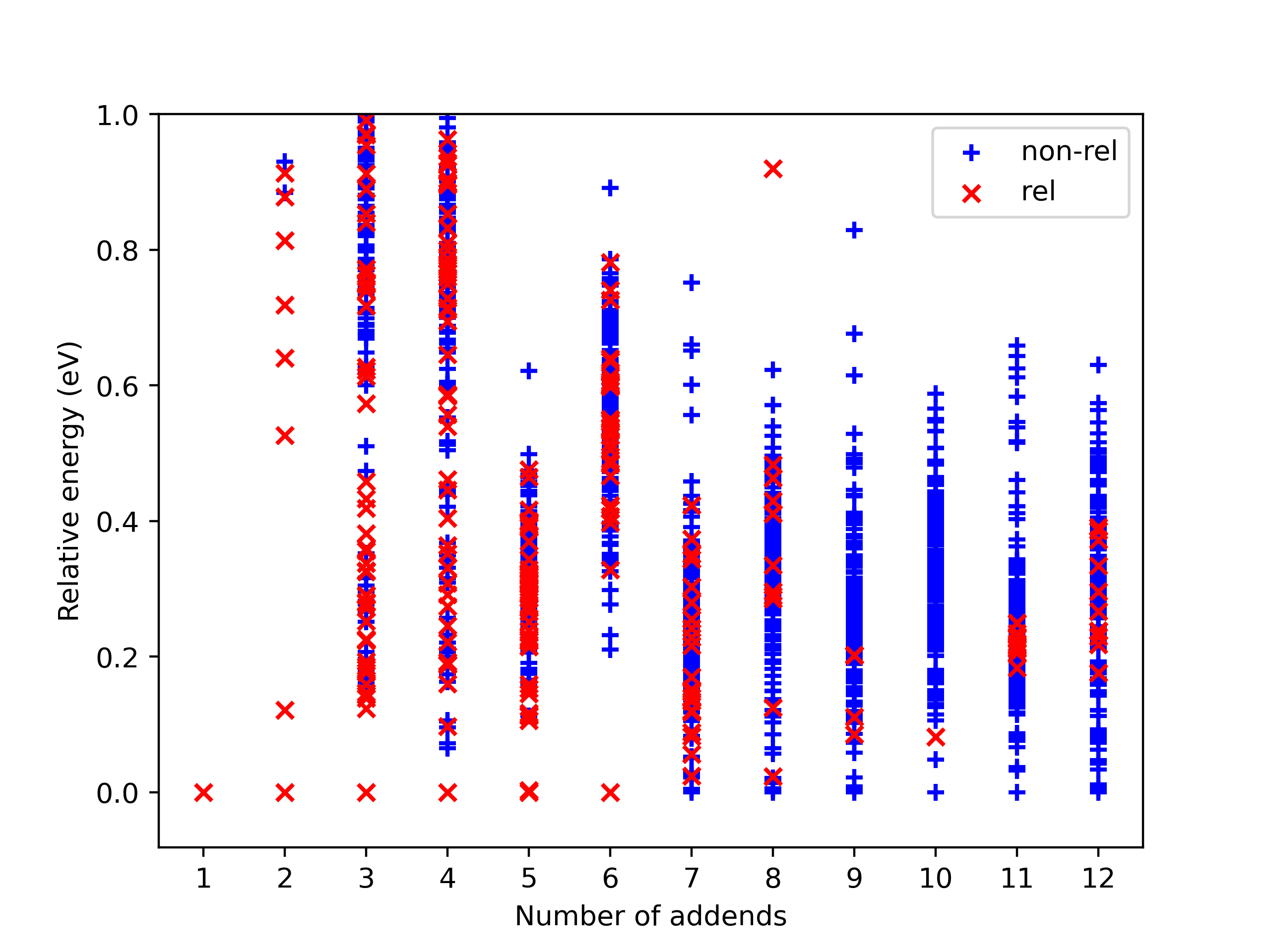
Fig 13. Example of the dumped information. The red ‘x’ presents a relative, blue ‘+’ is a non-isomerphic one.
In addition, AutoSteper dumps the relative energy of each scanned
isomer, and groups them into the non_rel_e and rel_e.
Collect failed
The failed-check optimization jobs are collected into the
failed_job_paths file. To have an overview of failed job types, call
function clc_failed.
Three parameters are required:
workbase: where the simulation is performed, see sectionSimulationModulesFig 2.dump_pic_path: where the collected information dumps, an absolute root to a picture.ylim: Optional parameter. For users who are interested to set an upper limit of the y-axis.
Fig 14 presents a collected distribution of failed jobs, it was performed with \(\rm C_{60}Br_x\) systems, 50 isomers for x = 3, 6, 9, 12, 15, 18 are sampled with AutoSteper’s random mode.
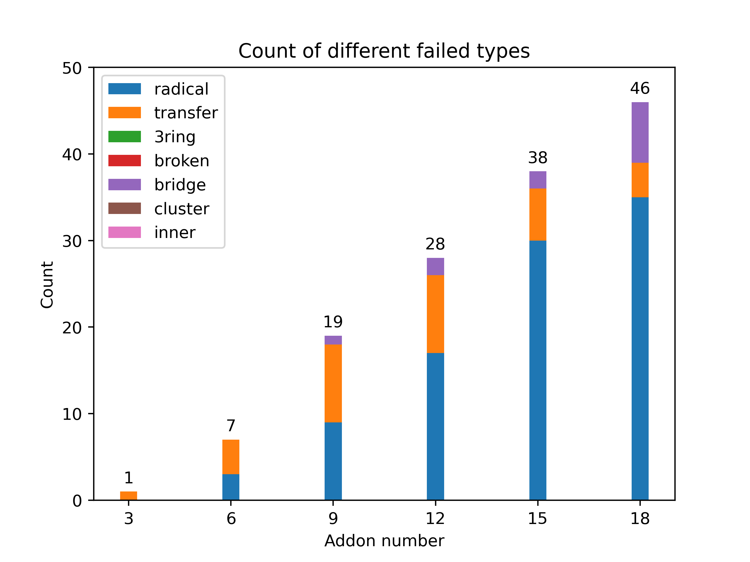
Fig 14. Distribution of failed jobs for a random simulation.
The legend on the upper left denotes the types of failed jobs. They are corresponding to the 7 rules mentioned in the previous section. See clc_failed.
Binding energy analysis
The binding energy well explains the reaction activity. Based on the
structured topological information provided by the cook_disordered
function, one can easily parse the binding energy information. Set
hydrofullerene as an example, AutoSteper following this equation to
calculate binding energy.
One needs provide the following parameters:
sorted_root: the structured source folder.cage_e: the energy of the pristine cage.addends_e: the energy of the simple substance of addons. Here in this case, its Hydrogen.
Note that, the cage_e and addends_e need to be calculated under
the same computational level as the general isomers.
The output of this function is dumped into the sorted_root/info/, in
the format of pickle and xlsx. For an example, see
binding_e.