Plot with FullereneDataParser
This section is for the visualization of isomers, pathways, and SWR
pairs in Schlegel diagram format. The autosteper.plotter module is
built on top of
FullereneDataParser,
which is an excellent tool designed and maintained by Yanbo Han, a
XJTU-ICP member. A vivid description of FullereneDataParser could be
found in: DOI:10.1039/D2CP03549A (XCSI: “Effect of orbital angles on the
modeling of the conjugate system with curvature”).
Note
Please cite the article: https://doi.org/10.1039/D2CP03549A, if autosteper.plotter is utilized in your work.
Basic usage
Plot a cage
Here is a standard workflow to plot a Schlegel diagram:
Prepare environment
import matplotlib.pyplot as plt
from autosteper.plotter import FullereneDataParser_Plotter
Prepare a coordinate containing object
A ase.Atoms object or a coordinate containing file:
from ase.build.molecule import molecule

C60 = molecule(name='C60')
Prepare a figure
This could be your customized figure, if this step is skipped, the plotter will set up a new figure with the parameters in below:
fig = plt.figure(figsize=[10, 10])
ax = fig.add_subplot(111)
Load cage into the figure
a_plotter = FullereneDataParser_Plotter()
a_plotter.load_cage(atoms=C60, ax=ax)
Save the picture
plt.savefig('customized_figure.png', dpi=400)
plt.close()
See:
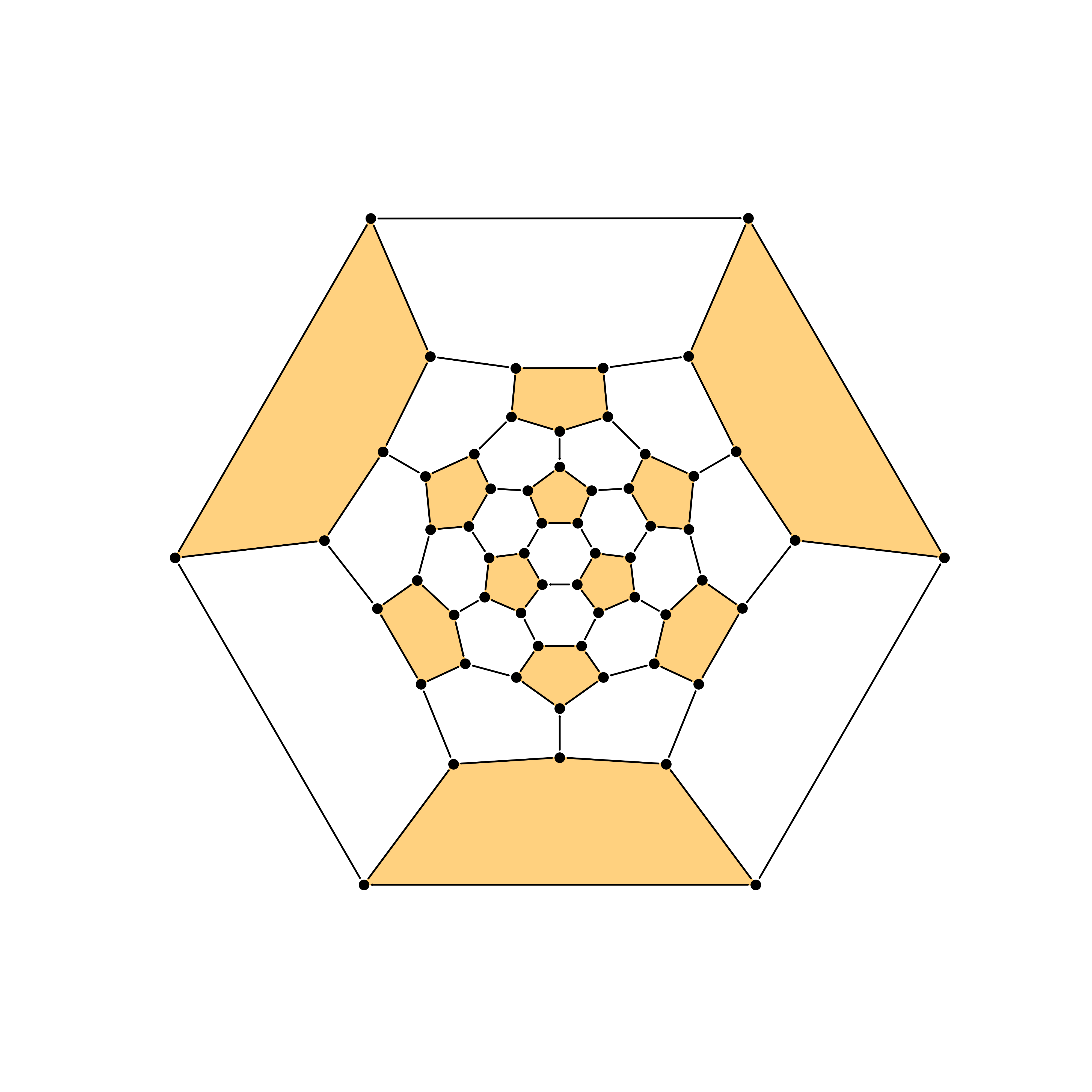
Fig 1. Schlegel diagram for C60.
Plot a C2nXm
Here is a simple way to plot Schlegel diagrams for C2nXm isomers.
Prepare packages:
import matplotlib.pyplot as plt
from autosteper.plotter import FullereneDataParser_Plotter
from autosteper.tools import strip_extraFullerene
Get the pristine cage and addon sites sequence
pristine_cage, addon_set = strip_extraFullerene(coord_file_path=r'dihept_C66H4.xyz')
Load cage and addon_set
a_plotter = FullereneDataParser_Plotter()
a_plotter.load_cage(atoms=pristine_cage)
a_plotter.load_addons(addon_set=addon_set, group_symbol='H')
Save pictures
plt.savefig('simple_plot.png', dpi=400)
plt.close()
See:

Fig 2. Schlegel diagram for C66H4.
Tailor your picture
There are multiple parameters in methods load_cage and
load_addons to help users to tailor the Schlegel diagram to their
own favor. Here present two cases to help users understand these
parameters.
Case 1: toggle projection ring
As we all know, classical fullerenes have pentagons and hexagons rings. The Schlegel diagrams are plotted by unzipping one ring and spreading the rest of the rings to a planar like a graphene nanosheet. Here we call the unzipped ring the projection ring. It will stay on the outmost side of the Schlegel diagram, and the opposite of this ring on the cage will become the center. FullereneDataParser can project from pentagons and hexagons, however, it’s not recommended to project from pentagons.
Here we take dihept-C66H4 for example. If not specified, FullereneDataParser will randomly choose a hexagon to project from. Result in Fig 2.
To specify a pleasant projection ring, one may start to see labels:
a_plotter.load_cage(atoms=pristine_cage, show_C_label=True, C_label_transparency=0.5, C_label_color='orange')
a_plotter.load_addons(addon_set=addon_set, group_symbol='H', show_addon_nums=True)
plt.savefig('plot_with_label.png', dpi=400)
plt.close()
See:
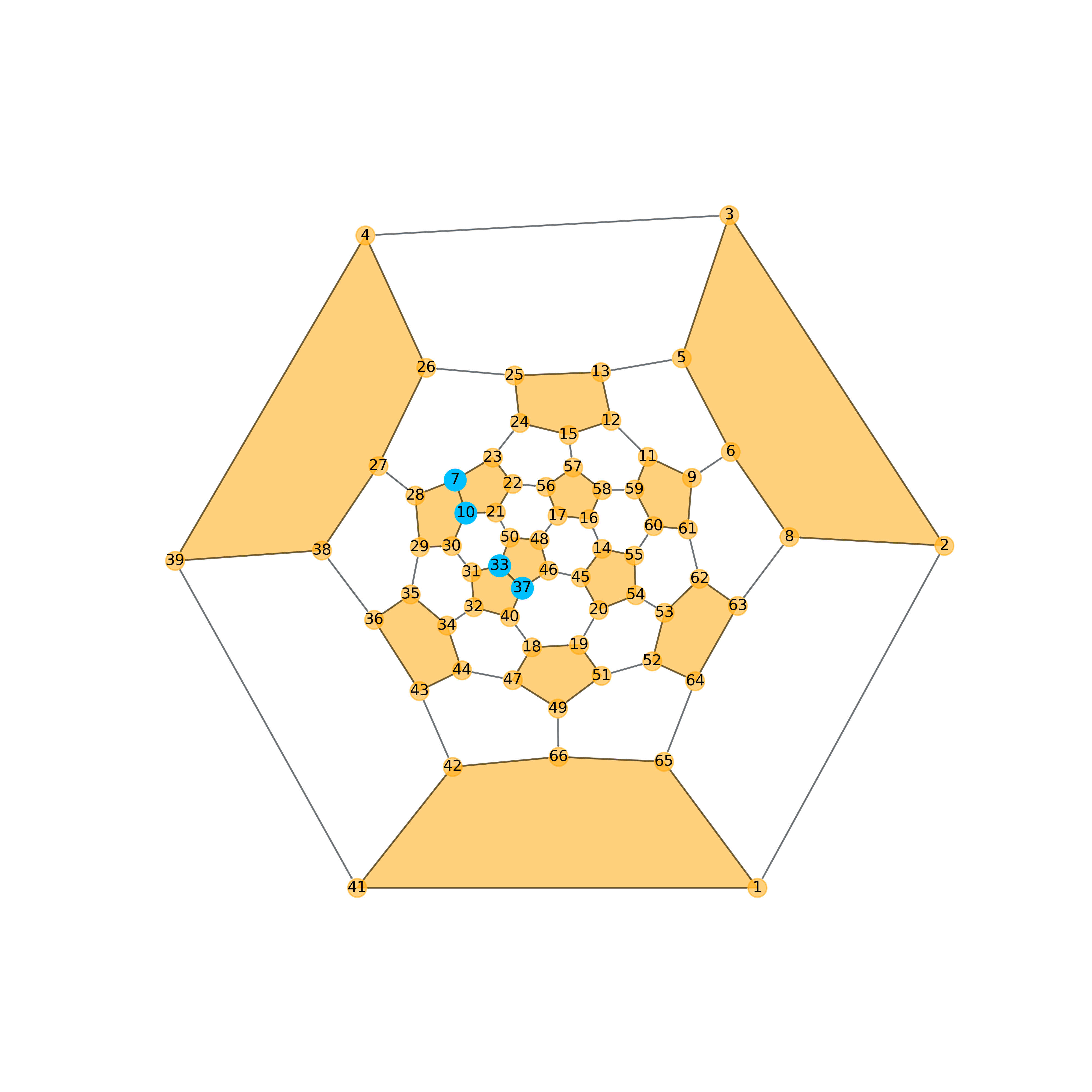
Fig 3. Schlegel diagram with labels for C66H4.
As one may notice, the [10, 30, 31, 33, 21, 50] ring connected two Adjacent Pentagon Pairs(APPs), to project from this ring will result in a symmetrical diagram:
a_plotter.load_cage(atoms=pristine_cage, show_C_label=True, C_label_transparency=0.5, C_label_color='orange',
                    proj_ring_seq=[10, 30, 31, 33, 21, 50])
a_plotter.load_addons(addon_set=addon_set, group_symbol='H', show_addon_nums=True)
plt.savefig('re_plot_with_label.png', dpi=400)
plt.close()
See:
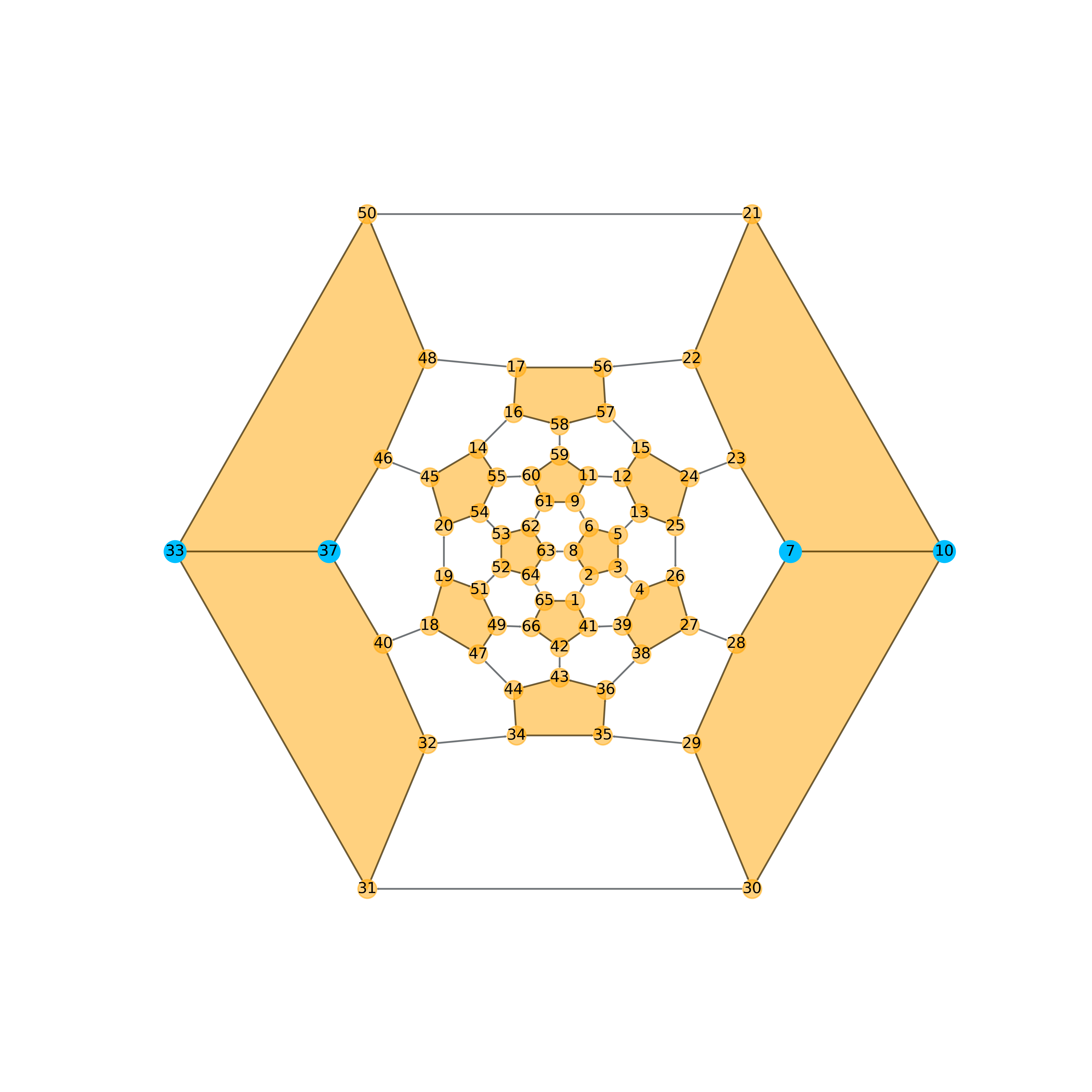
Fig 4. Re-plot schlegel diagram for C66H4.
Note that, the outmost ring has changed to [10, 30, 31, 33, 21, 50].
Finally, clean this picture:
a_plotter.load_cage(atoms=pristine_cage, proj_ring_seq=[10, 30, 31, 33, 21, 50])
a_plotter.load_addons(addon_set=addon_set, group_symbol='H')
plt.savefig('Clean.png', dpi=400)
plt.close()
See:

Fig 5. Clean schlegel diagram for C66H4.
Case 2: zoom in
As one may notice, pictures need to be scaled up for a pleasant view of labels (Fig 4 and Fig 5). A straightforward way to avoid scaling up the whole picture is to scale up fonts only. However, rings in the center may be too crowded for this operation.
Here we take \(\rm ^{\#4169}C_{66}Cl_{10}\) for example, to set default labels:
pristine_cage, addon_set = strip_extraFullerene(coord_file_path=r'C66Cl10_4169_exp.xyz')

a_plotter = FullereneDataParser_Plotter()
a_plotter.load_cage(atoms=pristine_cage, proj_ring_seq=[61, 62, 63, 64, 65, 66])
a_plotter.load_addons(addon_set=addon_set, group_symbol='Cl', show_addon_nums=True)

plt.savefig('default.png', dpi=400)
plt.close()
Labels are too small to see:
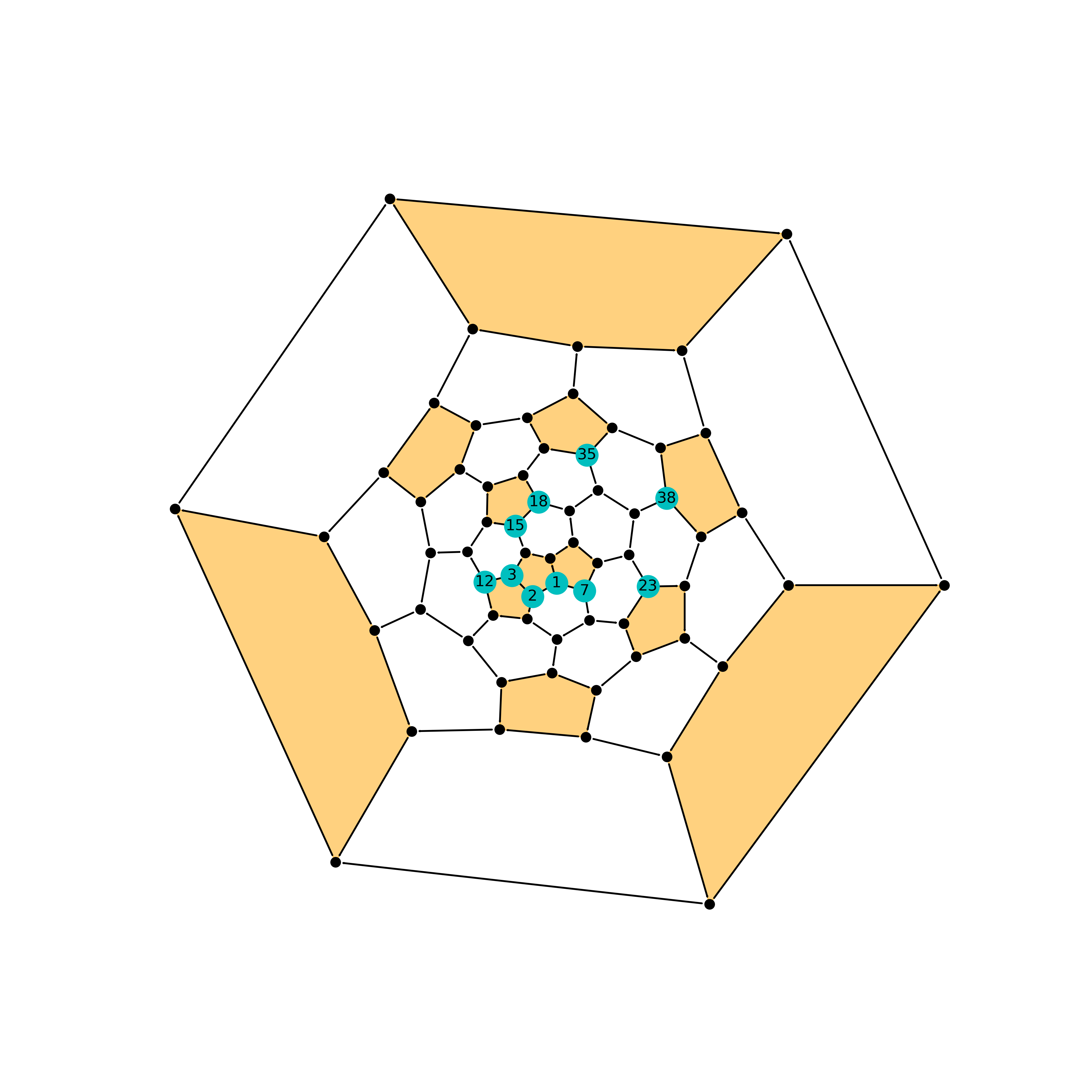
Fig 6. Default schlegel diagram for C66Cl10.
Scale up the font size and base circle:
a_plotter.load_addons(addon_set=addon_set, group_symbol='Cl', show_addon_nums=True, fontsize=25, addon_label_size=750)
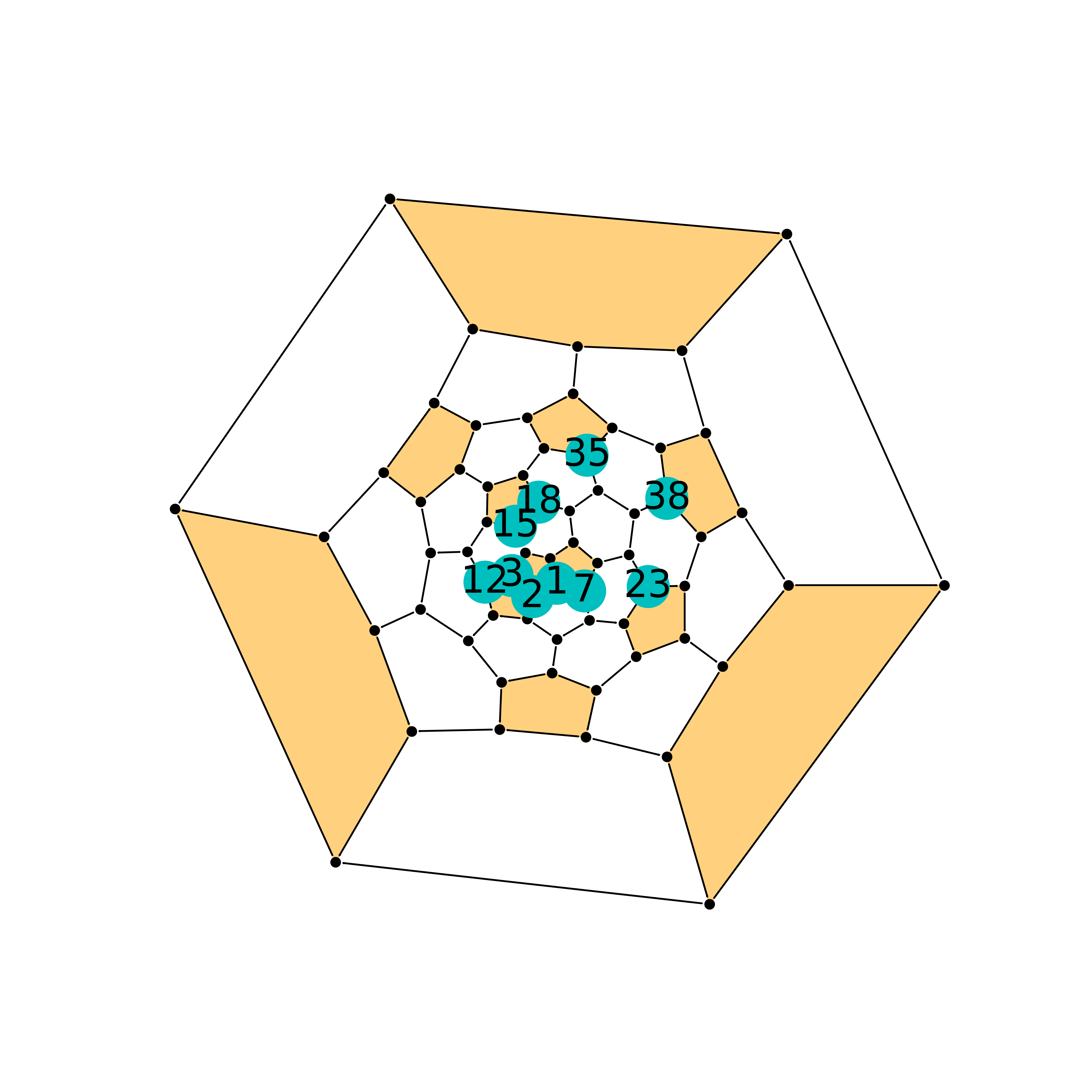
Fig 7. Scale font size only for C66Cl10.
It’s hard to see rings behind labels. Note that, we are focusing on the triple fused pentagons and the encircled hexagon in the center. However, the outside pentagons took the majority of the picture. If we zoom in like classical image processing tools, the center of the diagram will be enlarged. Following this track, one step further is that we want to zoom in on the center while squeezing outside rings.
To do that, one needs to toggle the sphere_ratio and parr_ratio
parameters. The two of them control the shape of the outer object that
will be projected onto. Generally speaking, the center will be zoomed in
if sphere_ratio is high. By default, sphere_ratio=0.8 and
parr_ratio=0.2. If we set sphere_ratio=6 and do not change
parr_ratio. That is:
a_plotter.load_cage(atoms=pristine_cage, proj_ring_seq=[61, 62, 63, 64, 65, 66], sphere_ratio=6)
The center of this image will be zoomed in like this:
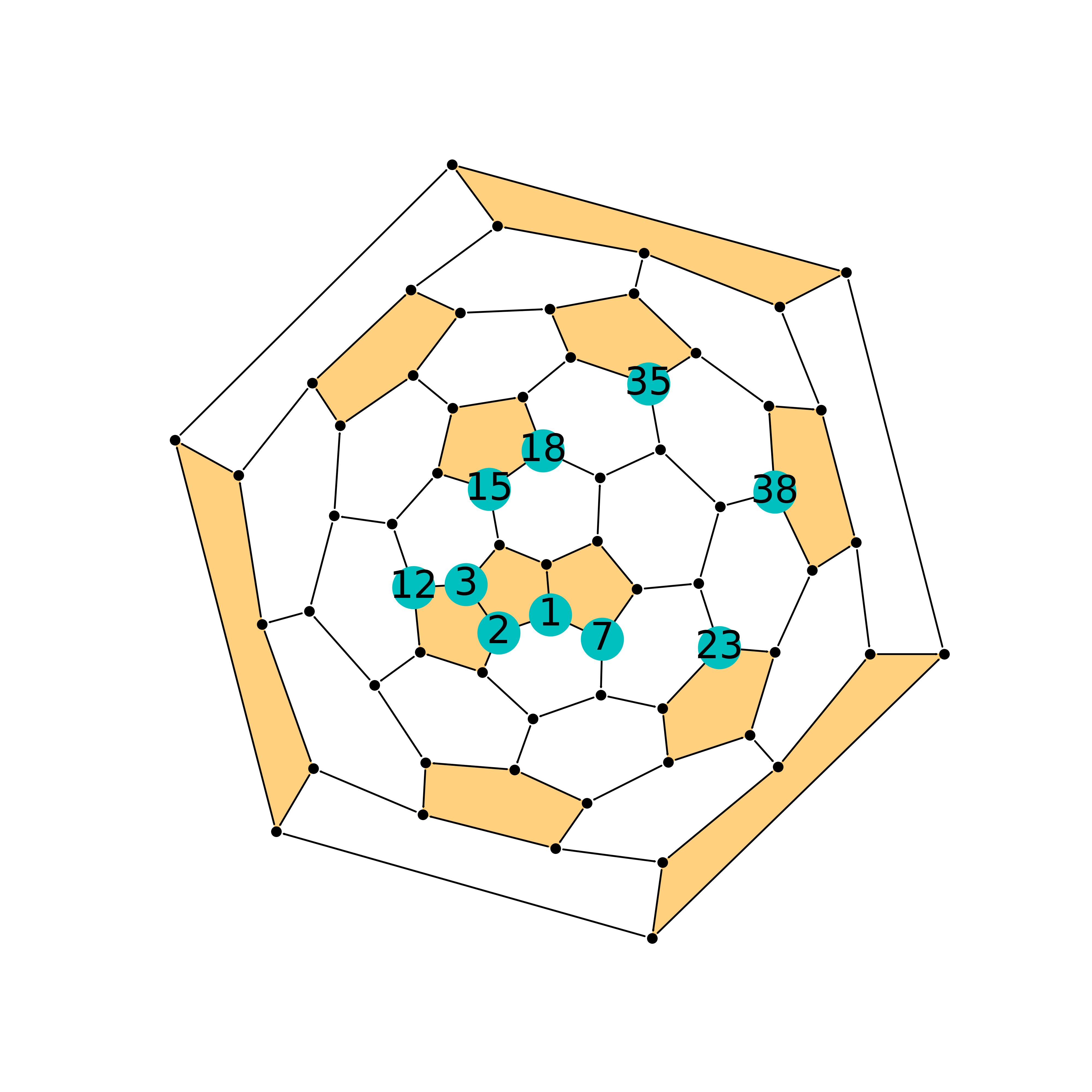
Fig 8. Zoom in for C66Cl10.
If one needs to replace these numbers with a more meaningful sequence
and rotate numbers to stay in line with the diagram,
addon_nums_rotation and replace_addon_map may be helpful:
original_seq = [1, 2, 3, 12, 7, 23, 38, 35, 18, 15]
new_seq = list(range(1, 11, 1))
replace_addon_map = dict(zip(original_seq, new_seq))

a_plotter = FullereneDataParser_Plotter()
a_plotter.load_cage(atoms=pristine_cage, proj_ring_seq=[61, 62, 63, 64, 65, 66], sphere_ratio=6)
a_plotter.load_addons(addon_set=addon_set, group_symbol='Cl', show_addon_nums=True, fontsize=25,
                      addon_label_size=750, addon_nums_rotation=-17, replace_addon_map=replace_addon_map)
This is the lowest-energy pathway of \(\rm ^{\#4169}C_{66}Cl_{10}\):
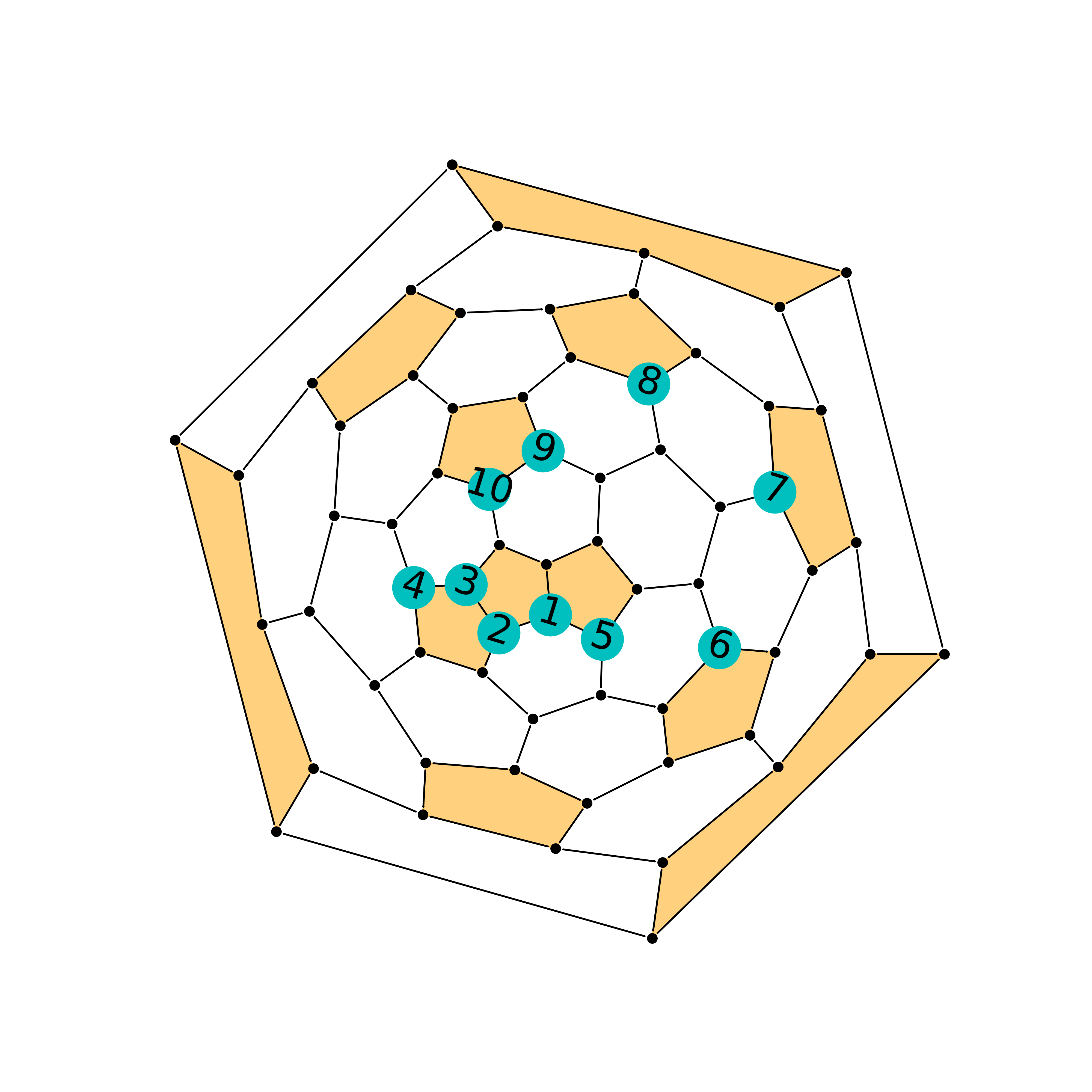
Fig 9. Lowest-energy pathway for C66Cl10.
Summary of parameters
load_cage parameters:
Prepare coordinates:
coord_file_path(str) oratoms(ASE Atoms format)About carbon atoms on the cage (the black dots):
C_label_color: by default, it’sblackC_label_transparency: by default, it’s solid 1show_C_label: show numbers on top of carbon atoms
Which ring to project from:
proj_ring_seq, set or list, start from 1About pentagons:
pentagon_color: by default, it’sorangepentagon_transparency: by default, it’s 0.5. This parameter is useful when projecting from pentagons, which will result in disaster, again, we do not recommend projecting from pentagons.
Zoom in:
sphere_ratio, parr_ratio: by default, it’s0.8:0.2, turnsphere_ratioup will zoom in.
ax: figure handle to plot, by default, a [10, 10] figure will set up.
load_addon parameters:
addon_set: cage sites that are functionalied by groups. (Caution: addon set start from 0)addon_color: color of addons on diagramgroup_symbol: symbol of groups, this will help to assign default colors ifaddon_colornot specified.addon_label_size: size of labelsshow_addon_nums: set true to see numbers of addonsaddon_nums_rotation: set true to rotate these numbersreplace_addon_map: a map to replace addon numbers
Plot low e isomers
A simple loop will do for good.
import matplotlib.pyplot as plt
from autosteper.plotter import FullereneDataParser_Plotter
from autosteper.tools import get_low_e_ranks, strip_extraFullerene
import pandas as pd


a_plotter = FullereneDataParser_Plotter()
# Here we take example on dihept-C66H4
info = pd.read_pickle(r'path/to/passed_info.pickle')
cutoff_para = {
    'mode': 'rank',
    'rank': 5
}
for a_rank in get_low_e_ranks(e_arr=info['energy'], para=cutoff_para):
    a_xyz_path = info['xyz_path'][a_rank]
    cage, addon_set = strip_extraFullerene(coord_file_path=a_xyz_path, group='H')
    a_plotter.load_cage(atoms=cage)
    a_plotter.load_addons(addon_set=addon_set)
    plt.savefig(f'rank_{a_rank+1}_2D.png', dpi=400)
    plt.close()
Plot pathways
To plot a pathway, the quick way is to directly plot each xyz file into
a 2D Schlegel diagram. This will indeed work for pathways generated from
Path_parser module since pathways are generated with strict sequence
matches. A [0, 1] addon sequence will have derivatives [0, 1, 2, 3], but
will never give [7, 8, 2, 3].
However, the cook disordered function re-generated topological
linkage information by solving sub-graph isomorphism problems. For
example, in Fig 10, C60Cl4-1 is isomorphic with C60Cl4-2. Both of them
could be precursors of C60Cl6. This will bring inconsistency for pathway
visualization.

Fig 10. Illustration of isomorphism problem.
To solve this problem, we need to re-label intermediates by matching their addon sequence to a subset of the end-addition-state one.
This will be good for a single pathway. When it comes to multiple pathways, a new problem will emerge if mixed end-addition-state isomers are involved. As mentioned above, we match intermediates to the end-addition-state isomer. Which one to map when there are multiple end-addition-state isomers?
Here we propose to match the lowest-energy one.

Fig 11. Illustration of re-match end-addition-state isomers.
Figure 11 (a) is the synthesized \(\rm ^{\#4169}C_{66}Cl_{10}\). Figure 11 (b) is the second lowest-energy isomer. One may notice that both of them have an encircled hexagon and their difference comes from the triple fused pentagons. However, this observation can only be achieved by experienced fullerene researchers. Visualization of the two could be prettified by matching mutual addon sites, see Figure 11 (c).
Dealing with these tricky matching problems has been wrapped into a
single method, plot_pathway_unit. For parameters:
src_pathway_root: the original pathway rootnew_pathway_workbase: new pathway workbaseis_match_max_adduct: set true to match max adduct to a specific isomermax_adduct_path: the path to the specific isomerdiff_len: how much shifts between two isomersis_re_label: set true to plot after re-labeldpi: the quality of dumped pictures
The rest of the parameters are the same as in the previous section.
Plot SWR
The problem of plot SWR is basically the same as above. A one-step-SWR between cage 1 and cage 2 means there is one C-C bond rotated 90 degrees in cage 1 to become cage 2.
For example, \(\rm ^{\#11}C_{84}\) and \(\rm ^{\#12}C_{84}\),
there are 82 identical carbon atoms. One needs to match pristine cages
before the load_cage stage and change the addon numbers to the new,
re-matched cages.
In the latest version of AutoSteper, this kind of cage-matching has been
wrapped into the find_SWR function. Information about SWR bonds and
addon sites has been dumped into the sites_info.txt. Therefore, the
plot section has been released from complex matching problem. Simply
plot every xyz file with regard to sites info well present a pleasant
view.
The corresponding method is plot_swr. For parameters:
src_swr_root: root to the AutoSteper-generated SWR pairsdpi: the quality of dumped pictures
Warning
If projection ring is specified, please make sure the projection ring is in the queried atoms. The target atoms is mapped to the queried atoms. There are some scenarios that this ring does not appear in the mapped target atoms. But it’s very rare. After all, be careful about this parameter!
The rest of the parameters are the same as in the previous section. This
method will navigate to the original SWR workbase(src_swr_root),
match pristine cages, plot, and dump pictures in that folder.
(The support for multi-step SWR is still under development.)
Figure 12 presents one of the scenarios:
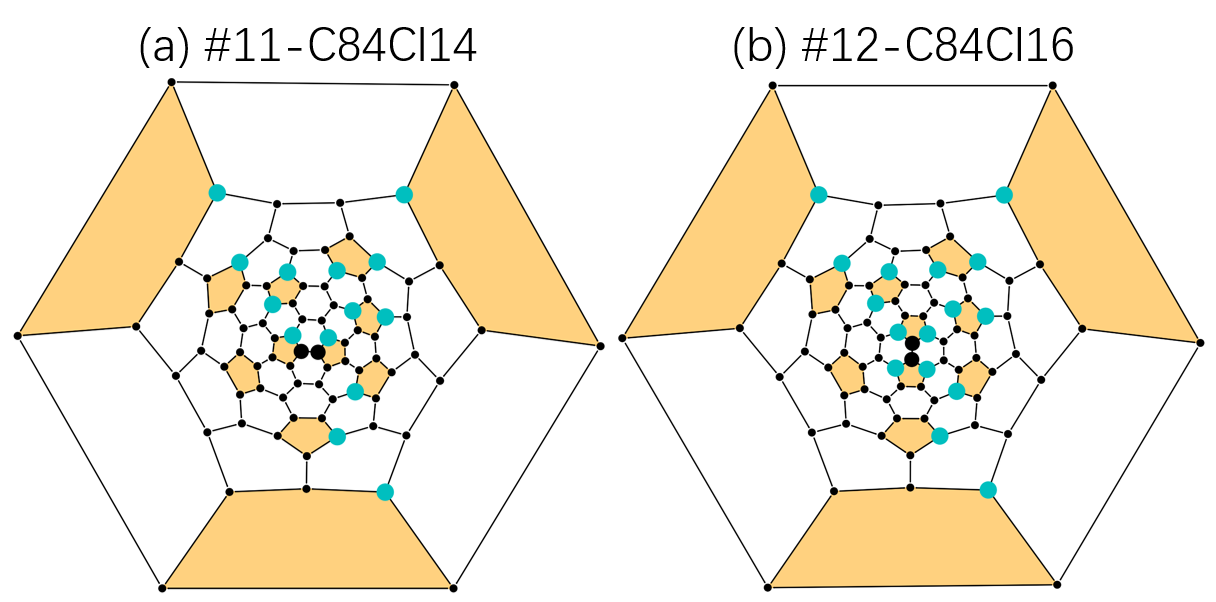
Fig 12. Illustration of an AutoSteper-generated SWR pair.
The two bold carbon atoms are the rotated C-C bond.