Simulation Modules¶

AutoSteper provides a fully automated fashion to simulate stepwise chemical reactions. That contains on-the-fly building, optimizing, and checking. Additionally, a light-weight pathway search algorithm is built along with the simulation, and some variants of the stepwise model are proposed in pre-san and blacklist sections. In the end, we will address some engineering problems.

AutoSteper¶

AutoSteper is the highest level of abstraction. It controls sub-modules to simulate the entire stepwise addition process. It has 3 different modes, corresponding to the 3 generator’s modes. Details are presented below:

step: the stepwise simulation.
random: randomly generate isomers and optimize them to an equilibrium state.
base: enumerate and evaluate all the non-isomorphic isomers for a specific addon number.

Here brings a gentle introduction to three of them.

step¶

Input script¶

Here is one of the typical input script:

import os

from autosteper import AutoSteper

mach_para = {
    'batch_type': "Torque",
    'context_type': "LocalContext",
    'remote_root': 'x/to/test_dpdispatcher',
    'remote_profile': None
}

resrc_para = {
    'number_node': 1,
    'cpu_per_node': 6,
    'gpu_per_node': 0,
    'group_size': 10,
    'queue_name': "batch",
    'envs': {
        "OMP_STACKSIZE": "4G",
        "OMP_NUM_THREADS": "3,1",
        "OMP_MAX_ACTIVE_LEVELS": "1",
        "MKL_NUM_THREADS": "3"
    },
    'sub_batch_size': 50
}

para = {
    'pristine_path': r'C60.xyz',
    'root': r'./',
    'gen_para': {'group': 'Cl',
                 'geom_mode': 'pre_defined',
                 'gen_core_path': r'path/to/cagesearch'
                 },
    'opt_mode': 'xtb',
    'opt_para': {
        'has_parity': True,
        'cmd_list': [r'path/to/xtb', '--opt', 'tight', '--json'],
        'out_list': ['xtbopt.xyz', 'xtbopt.log', 'xtbout.json'],
        'deal_wrong_mode': 'Report',
        'mach_para': mach_para,
        'resrc_para': resrc_para,
    },
    'run_para': {
        'start': 1,
        'stop': 3,
        'step': 1,
        'wht_list_para': {
            'mode': 'rank',
            'rank': 3
        }
    },
}

auto = AutoSteper(para=para)
auto.run()

An example could be found in test_step.

Parameters and folder system¶

The resrc_para and mach_para are designed to configure a suitable environment for optimizers. (see optimizer module) After that, one needs to configure the parameter of the class AutoSteper. Specifically, one needs to provide:

pristine_path: the path to the pristine cage. It could be in any mainstream structure format, only if the ASE package supports it.
root: the ABSOLUTE path to the growth simulation workbase, where the AutoSteper would make a directory in the name of the pristine cage. Fig 1 presents one of the workbase directory.

Fig 1. An AutoSteper workbase.

The gen_para and opt parameters configure a generator and an optimizer. To simulate a stepwise addition reaction, one needs to provide the run_para with the following parameters considered.

start: the addition stage (\(\rm C_{2n}X_{start}\)) when the simulation started. The first step will enumerate and evaluate all the non-isomorphic isomers without any filter.
stop: the addition stage (\(\rm C_{2n}X_{stop}\)) when the simulation started.
step: number of the newly attached functional groups after the first step.
wht_list_para: parameters to control the isomers saved in every step. These isomers will serve as seeds in the next step to generate derivatives. Details see next section.

AutoSteper would create sub-workbases for every addon number. Fig 2 presents one of the scenarios. In this case, the start value is 1, the stop value is 10, and the step value is 1.

Fig 2. An AutoSteper sub-workbase.

The directory of the first step is illustrated in Fig 3.

Fig 3. The first step workbase.

The functions of each file/directory are presented below.

raw: the quasi-equilibrium isomers built in every step.
cooked: the equilibrium state of each isomer, in xyz format.
cooking: the real workbases for each optimization job. It typically contains more optimization details than the cooked folder.
failed_job_paths: the absolute path of each failed optimization job as well as their corresponding failed status code.
geom_1_addons.out: the enumerated addition patterns in the first step. geom is the name of the pristine cage, 1 is the addon number of the first step.
passed_info.pickle: key information of the optimization jobs that passed the topological check. In the early version of AutoSteper, this file is called deep_yes_info.pickle, meaning information is stored in a deep chart. Fig 4 presents one of the scenarios. The meaning of each column is presented below:
- name: the name for each isomer, in 36 format.
- energy: the equilibrium energy of each isomer, in units eV.
- xyz_path: the absolute path to each isomer structure, in xyz format.
- nimages: the number of images in each optimization trajectory.

Fig 4. Example of the passed_info.

passed_info.xlsx: excel format of passed_info.pickle, up to 1000 items stored.
parent_info.pickle: key information of the parent-son relationships generated during the growth simulation. In the early version of AutoSteper, this file is called flat_yes_info.pickle, meaning information is stored in a flat chart, and only the passed isomers are considered. The flat format enables a fast index when parsing the topological information.
- The first step is different from others since there is only one parent for all the \(\rm C_{2n}X_{start}\) isomers. Fig 5 presents one of the cases. The columns correspond to each \(\rm C_{2n}X_{start}\) isomer. The first row corresponds to their energy.
- Fig 6 presents a case in the proceeding addition stages. The columns correspond to each \(\rm C_{2n}X_{m}, m>start\) isomer. The first row stores the names of their parent(s). Note that, isomers in \(\rm C_{2n}X_{m}\) addition stage could have more than one parent \(\rm C_{2n}X_{m-step}\). The second row corresponds to their energy.

Fig 5. Example of the parent_info in the first step.

Fig 6. Example of the parent_info in the proceeding addition stages.

status_info.pickle: the status code for each optimization job, in flat chart format for indexing convenience. Three types of status codes are reported:
- 0: normal termination.
- -2: wrong jobs. This would happen when there are no files retrieved from computational resources, for example, the internet is broken, or the initial structure is so unphysical that the optimizer program went broken.
- >0: the optimized isomer did not pass the topological check, their corresponding failed status codes will be reported. See the Checker section.

Fig 7. Example of the status_info.

An example about the co-occurrences of failed and wrong could be found in test_random. This module helps to maintain stable operation of the entire program.

The directory of the proceeding addition stages is illustrated in Fig 8. The difference compared with the first step is presented below:

sub_nauty: there is more than one parent that generates derivatives. Related information is dumped in this folder.

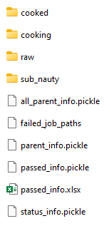
Fig 8. The workbase for the proceeding addition stages.

all_parent_info.pickle: the parent-son information for all the \(\rm C_{2n}X_{m}\) isomers. (see Fig 9.) This is generated when building the quasi-equilibrium isomers. Note that the parent_info.pickle only considers the passed ones, and it contains energy info. The all_parent_info.pickle stores duplicated but more detailed information, therefore it may be useful for future development.

Fig 9. Example of the all_parent_info.

Cut-off¶

Generally speaking, there are two types of cutoff. The hard one, rank, and the soft one, value.

The reason to call rank as hard is that, for each step, there are tens of thousands of isomers to be screened. We cannot estimate the sparsity of low-energy isomers beforehand. We can only set an upper limit base on our computational resources. It could be 200, or if one has 5 times the computational resources, this figure could be toggled to 1000. It’s tunable.

On the other hand, from a chemical view, one needs to set this cutoff with a soft criterion, value. This figure could be 1eV or other numbers. It’s tunable.

AutoSteper provides 4 modes to control the cutoff process:

rank
value
rank_or_value or value_or_rank: both of the cutoffs need to be met.
rank_and_value or value_and_rank: met anyone of the two cutoffs is sufficient.

In the latest version of AutoSteper, the default cutoff has been removed. Users MUST provide a reasonable energy cutoff for growth simulation. Here are two tips for users to choose a suitable cutoff:

The combination of rank and value cutoff may provide chemically intuitive and computationally affordable results.
A small cutoff is encouraged to perform a trial calculation, to ‘feel’ the computational cost, then enlarge it to gain a more complete view.

For input format, please check the example.

Another application of this function is to extract low-energy isomers from an information pickle file, see get_low_e_xyz.py.

random¶

The random mode could be used to sample targeted configuration space, for example, building a dataset to train Neural Network Potential (NNP). The parameters for random mode are basically the same as the step mode. Differences lie in the run_para, which is replaced by random_para. Specifically, one needs to provide:

addon_list: a list that consists of desired addon numbers, e.g, \(\rm C_{2n}X_{m}, m\ in\ addon\_list\).
random_num: for each addon number m, the number of randomly sampled isomers \(\rm C_{2n}X_{m}\).
try_times: since some systems are highly unstable, e.g, \(\rm C_{2n}X_{m}, m=2n\), all the isomers sampled could be unphysical and fail the topological check. In this case, the whole batch of isomers \(\rm C_{2n}X_{m}\) should be discarded. This parameter is highly recommended to control the failed chances. Note that, it needs deal_wrong_mode set as Tough to properly function.

Despite these parameters, the execution method of AutoSteper changed from run to random. For an example script, see test_random.

base¶

The base mode could be used to enumerate and evaluate all isomers for a specific system \(\rm C_{2n}X_{m}\). In fact, it could be viewed as the first step in the step mode. Since the base mode has only one step, its input script doesn’t need run_para. The rest of the parameters stay the same as above. The execution method of AutoSteper changed from run to base. For an example script, see test_base.

Generator¶

AutoSteper builds molecules with simple geometry techniques considered. See Fig x.

Fig x. Visualization of modeling techniques.

That is when one is trying to functionalize a carbon site. Three of its neighbors and the cage center are considered, see Fig x (a). To start with, here we put one Cl atom on top of this carbon site. This procedure is split into 3 steps:

Calculate the normal vector of the three neighbors formed plane.
If this normal vector points to the inside of this cage (judged by the cage center), give it a minus sign to make sure it points to the outside.
Start from the ‘to-be-functionalized’ atom, following the direction of the normal vector, at a distance of bond length, put an atom.

This will get a quasi-equilibrium isomer since the bond length is hand-tuned.

For the -OH group, an additional step is required:

Create a new atom. Set the distance between new atoms and previously defined O atom as a fixed value. Set the angle between new-O-C to a fixed value.

This will ensure that the new H atom is staying in a circle, its position will ensure that O-H distance and C-O-H met requirements, though its specific position will not be defined.

For the -CH3 and -CF3 group, an additional step is required compared to -OH:

After we put the first H or F atom, rotate the C-H (C-F) vector with the normal vector as the axis, \(\rm \frac{2}{3\pi}\) and \(\rm \frac{4}{3\pi}\) respectively to get two new vectors. Start from the new carbon atom, following these two vectors, at a distance of C-H (C-F) bond length, put the rest two atoms.

Details of parameters are presented below:

group: the name of functional groups. Currently, AutoSteper supports \(\rm C_{2n}X_m(X=H, F,Cl, Br, I, OH, CF_3, CH_3)\).
gen_core_path: the absolute path to the executable binary file cagesearch, which is compiled from the Franklalalala/usenauty repository.
geom_mode: decides how to build quasi-equilibrium isomers. This parameter is highly recommended to be set as pre_defined. The pre-defined geometry parameters are achieved from thousands of randomly sampled isomers. If one needs to change these parameters, set geom_mode to another value and assign new parameters through geom_para. Note that, the new format needs to stay consistent with the original.
skin: parameter to decide whether two atoms are bonded. For details see the checker module. By default, this parameter is set to be 0.15.

Note that, the generator module could be used alone to build hand-tuned structures. See build_unit.

Optimizer¶

The optimizer module heavily rely on open-source package deepmodeling/dpdispatcher. See Getting Started to get familiar with dpdispatcher. Here presents the usage of AutoSteper’s customized version.

machine and resource¶

To start with, one needs to set a machine and a resource configuration. Here present some examples.

For the machine parameter, two sets of configurations are recommended. See below:

# from local (typically your win system) to clusters. Input scripts are submitted in Personal Computer (PC).
mach_para = {
    'batch_type': "Torque",  # my cluster type
    'context_type': "SSHContext",
    'remote_root': '/home/test/xx/',  # the remote workbase where the actual computation take place.
    'remote_profile': {
        "hostname": "2xx.2xx.xx.7x",  # IP
        "username": "xx",
        "password": "xx",
        "port": 22,
        "timeout": 10
    }
}

# inside your clusters. Input scripts are submitted in the cluster.
mach_para = {
    'batch_type': "Torque",  # my cluster type
    'context_type': "LocalContext",  # Do not need IP information
    'remote_root': '/home/test/xx/',
    'remote_profile': None
}

For the resource parameter, here is an example:

resrc_para = {
    'number_node': 6, # the sequence name for your cluster.
    'cpu_per_node': 6, # computational resources for each task.
    'gpu_per_node': 0, # same as above
    'group_size': 10, # number of tasks contained in each job (group).
    'queue_name': "batch", # queue name for my cluster
    'envs': {              # extra enviromental variables
        "OMP_STACKSIZE": "4G",
        "OMP_NUM_THREADS": "3,1",
        "OMP_MAX_ACTIVE_LEVELS": "1",
        "MKL_NUM_THREADS": "3"
    },
    'sub_batch_size': 50 # number of tasks contained in each batch.
}

The machine parameters tell the dpdispatcher which cluster to use and how to contact, while the resource parameter assigns computation resources to each job.

The original workflow of the dpdispatcher is illustrated in Fig 10.

Fig 10. Simplified workflow of dpdispatcher.

Each optimization job corresponds to a task. Then, tasks are grouped (group_size) into jobs. These jobs are submitted through ssh or local context (context_type) to remote (remote_root), where the remote would assign computational resources to each job (All_cpu_cores /cpu_per_node) and execute them in parallel.

However, when it comes to huge task sequences, the number of groups in line may put pressure on the cluster. And when something wrong happened in a single job, the whole batch would be undermined. (For example, no retrieval from remote.) Therefore, we proposed the sub_batch_size parameter to perform job dispatch in a mini-batch style. An illustration of the modified dpdispatcher is presented in Fig 11.

Fig 11. A top-down illustration of the modified dpdispatcher.

More details could be found in the documentation of Machine parameters and Resources parameters.

opt mode and parameter¶

Currently, AutoSteper provides interfaces for 3 software, namely, the xTB program, the Gaussian software, and the ASE python library. In addition, AutoSteper provides the Multi_Optimizer to properly integrate different software or employ the same software repeatly. Examples could be found in optimizers.

The details about related parameters are presented below:

opt_mode: tells the AutoSteper class or the switch_optimizers function which optimizer to choose.
cmd_list: the actual command line in the final workbase (without the filename). It consists of the call of the program, options, flags, and so on.
out_list: the names of output files that need to be downloaded.
deal_wrong_mode: how to deal with wrong jobs, details see the engineering section.
has_parity: The spin multiplicity is different between odd and even addon number isomers. Set this button true if you intend to simulate odd addon number isomers. This will enabling an automated multipicity check.

Checker¶

The checker module will check optimized isomers to ensure an undermined topology. We implement the natural_cutoffs to decide whether two atoms are bonded.

Following this convention, we will assign covalent radii to each atom. For carbon atoms, it is 0.76, and for Cl atoms, it is 1.02.

Additionally, we assign each atom ‘skin’. That is, a fixed value for all atoms to boost the covalent radii. By default, this value is set to 0.3. That means for the carbon atom, the covalent radii raised to 1.06, and for Cl atoms, it’s 1.32.

With these parameters, if a carbon atom is within a 1.06+1.32(2.38) distance, we will decide they are bonded. However, the Cl-cage bond length distribution show that, the distance is around 1.8, see Fig x. Therefore, we turned down the skin value to 0.15. This will set a 2.08 bond length limitation.

Fig x. The distribution of Cl-Cage bond length.

Note that, if a Cl atom deviated from the equilibrium position. The optimizer will either put this atom into another equilibrium position or turn it into a radical. It’s rare that this atom will stay in bonding boundaries.

The skin parameter is tunable for a loose or tight bonding criterion.

7 scenarios could be detected, their corresponding failed status codes are presented below.

1: At least one functional group breaks the bond with the cage and becomes a radical.
2: At least one functional group deviates from the initial addition site and moves to another.
3: At least one 3-membered carbon ring is formed during optimization, meaning the pristine cage is squeezed by functional groups.
4: At least one carbon atom only has 2 neighboring carbon atoms or less, meaning the cage is broken.
5: At least one functional group binds with 2 or more carbon atoms, which is unstable for currently supported functional groups.
6: At least one carbon atom binds with 5 or more atoms, which means a small cluster or a coordination is formed.
7: The inner intactness of at least one functional group (\(\rm OH, CF_3, CH_3\)) is undermined.

Here in Fig x, we present examples:

Fig x. Illustration of some of the failed types.

These status codes will be reported in the failed_job_paths file and could be indexed from the status_info.pickle. Additionally, these status codes could be collected with help of clc_failed function, see Analysis Functions section.

Need to mention that, the AutoSteper module doesn’t need any specific input parameters for the checker module, though it could also be used alone. See checker.

Black list¶

The concept of the blacklist is based on the assumption that high-energy isomers probably contain local instability motifs, therefore their derivatives will unlikely to become stable ones since they still contain those instability motifs. This is a dual concept to the low-energy configuration space, which is treated as seeds to generate derivatives. See Fig 13.

AutoSteper collects two kinds of isomers into the blacklist.

The isomers that failed the topological check. (denote as failed)
The high-energy isomers within certain reverse cutoff. (denote as unstable)

Fig 13. Illustration of the high-energy configuration space.

When it comes to a new step, the new addition patterns will check through the blacklist at first. If a pattern contains any of the recorded patterns, it will be directly skipped.

To control the influence of a high-energy pattern, AutoSteper provides a queue to store high-energy patterns. See Fig 14.

Fig 14. Illustration of the queue maintained by AutoSteper.

AutoSteper starts collecting high-energy isomers in start_clct_num. These patterns start functioning in the next step and will continue to function till start_clct_num+container_size*step. The blacklist system will shut down after final_chk.

To enable the blacklist feature, one needs to provide a blk_para. Here is an example of blk_para, for example of an input script, see black_list.

blk_para = {
    'start_clct_num': 2,
    'final_chk_num': 8,
    'clct_unstb': True,
    'unstb_para': {
        'mode': 'rank',
        'rank': 10,
    },
    'container_size': 3
}

Note that, all failed addition patterns are collected by default as long as the blacklist system functions. Another kind of high-energy isomers is collected when the clct_unstb is Ture. The unstb_para controls the reversed cutoff range, details see test_cutoff.

Pre-scan¶

The pre-scan feature takes the quasi-equilibrium geometry to approximate the equilibrium state isomer. Since AutoSteper builds quasi-equilibrium isomers in a python environment, currently only the python package ASE is supported as the single-point evaluator.

The generated isomer (in atom class) would go through a single-point evaluation before dumping to a xyz format file. After the generation of all isomers, the low-energy ones will be selected and re-dumped into the post_pre_scan_raw folder. These isomers would undergo geometry optimization with optimizers. Fig 15 presents a working folder when the pre-scan feature is enabled. It’s basically the same as the step mode workbase.

Fig 15. The workbase when the pre-scan feature enabled.

To enable a pre-scan feature, one needs to provide a pre_scan_para. Here is an example of pre_scan_para, for example of an input script, see test_pre_scan.

pre_scan_para = {
    'start_ps_para': 2,  # when the pre-scan feature enabled
    'final_ps_para': 3,  # when the last addition stage that the pre-scan feature functions
    'calculator': calculator, # the calculator in ASE format
    'ps_cut_para': {     # to control the cutoff range
        'mode': 'rank',
        'rank': 80
    }
}

Note:

The calculator needs to stay in ASE format.
The ps_cut_para controls the cutoff range for the isomers that need geometry optimization.

Engineering¶

Currently, AutoSteper provides restart and error_handling for engineering convenience. More features are under development.

restart&proceed¶

The restart feature is designed for the step mode in case the simulation is interrupted. To use it, simply replace the execution method of AutoSteper to restart. For example:

# auto.run()
auto.restart(restart_add_num=5)

Note that, the restart method will delete the original workbase for \(\rm C_{2n}X_{m}, m>= restart\_add\_num\), after that, a new workbase will be created for \(\rm C_{2n}X_{m}, m= restart\_add\_num\). Make sure the restart_add_num equals the exact to addon stage when the simulation was interrupted.

Besides, this feature could be used to proceed with a normally terminated simulation. For example, the original one terminated in add_num = 4, and the restart_add_num could be set as 4+step. See test_restart.

error handling¶

The error_handling feature is assigned to optimizers. For description convenience, details of them are presented in this section. Note that, the error mentioned here denotes an unexpected optimization task result, which is different from the failed notation.

There are 4 modes in total. Specifically:

Report: simply report the wrong information and end out.
Complete: recursively submit jobs in small batches to minimize the wrong jobs, then end out. Note that, the dpdispatcher submits jobs in a batch style. When there is one job ends unexpectedly, there would be no retrieval from the remote for the whole batch. The Complete mode will submit recursively with small batches until the abnormal ones are left.
Tough: designed for random mode in case the whole batch of randomly generated isomers are unphysical. The old batch will be discarded and a new batch will be generated.
Ignore: designed for random mode in case there are abnormally terminated jobs. There will be warnings while the simulation proceeds.

Examples about how this feature function is presented in test_random.